Statistical Rethinking 2nd edition Homework 9 in INLA
library(tidyverse)
library(rethinking)
library(dagitty)
library(INLA)
library(knitr)
library(stringr)
1. data(Primates301) measurement error: INCOMPLETE
Consider the relationship between brain volume (brain) and bodymass (body) in the data (Primates301). These values are presented as single values for each species. However, there is always a range of sizes in a species, and some of these measurements are taken from very small samples. So these values are measured with some unknown error.
We don’t have the raw measurements to work with—that would be best. But we can imagine what might happen if we had them. Suppose error is proportional to the measurement. This makes sense, because larger animals have larger variation. As a consequence, the uncertainty is not uniform across the values and this could mean trouble.
Let’s make up some standard errors for these measurements, to see what might happen. Load the data and scale the the measurements so the maximum is 1 in both cases:
library(rethinking)
data(Primates301)
d <- Primates301
cc <- complete.cases( d$brain , d$body )
B <- d$brain[cc]
M <- d$body[cc]
B <- B / max(B)
M <- M / max(M)
Now I’ll make up some standard errors for B and M, assuming error is 10% of the measurement.
Bse <- B*0.1
Mse <- M*0.1
Let’s model these variables with this relationship: Bi ∼ Log-Normal(μi, σ) μi =α+βlogMi
This says that brain volume is a log-normal variable, and the mean on the log scale is given by μ. What this model implies is that the expected value of B is: E(Bi|Mi) = exp(α)Mi^β
So this is a standard allometric scaling relationship—incredibly common in biology.
Ignoring measurement error, the corresponding ulam model is:
dat_list <- list( B = B,
M=M)
m1.1 <- ulam(
  alist(
B ~ dlnorm( mu , sigma ),
mu <- a + b*log(M),
a ~ normal(0,1),
b ~ normal(0,1),
sigma ~ exponential(1)
) , data=dat_list )
##
## SAMPLING FOR MODEL '2bcae94530709687a15da757cbb5d4b7' NOW (CHAIN 1).
## Chain 1:
## Chain 1: Gradient evaluation took 3.1e-05 seconds
## Chain 1: 1000 transitions using 10 leapfrog steps per transition would take 0.31 seconds.
## Chain 1: Adjust your expectations accordingly!
## Chain 1:
## Chain 1:
## Chain 1: Iteration: 1 / 1000 [ 0%] (Warmup)
## Chain 1: Iteration: 100 / 1000 [ 10%] (Warmup)
## Chain 1: Iteration: 200 / 1000 [ 20%] (Warmup)
## Chain 1: Iteration: 300 / 1000 [ 30%] (Warmup)
## Chain 1: Iteration: 400 / 1000 [ 40%] (Warmup)
## Chain 1: Iteration: 500 / 1000 [ 50%] (Warmup)
## Chain 1: Iteration: 501 / 1000 [ 50%] (Sampling)
## Chain 1: Iteration: 600 / 1000 [ 60%] (Sampling)
## Chain 1: Iteration: 700 / 1000 [ 70%] (Sampling)
## Chain 1: Iteration: 800 / 1000 [ 80%] (Sampling)
## Chain 1: Iteration: 900 / 1000 [ 90%] (Sampling)
## Chain 1: Iteration: 1000 / 1000 [100%] (Sampling)
## Chain 1:
## Chain 1: Elapsed Time: 0.095752 seconds (Warm-up)
## Chain 1: 0.078632 seconds (Sampling)
## Chain 1: 0.174384 seconds (Total)
## Chain 1:## Warning: Tail Effective Samples Size (ESS) is too low, indicating posterior variances and tail quantiles may be unreliable.
## Running the chains for more iterations may help. See
## http://mc-stan.org/misc/warnings.html#tail-essprecis( m1.1 )
##            mean         sd      5.5%     94.5%    n_eff    Rhat4
## a     0.4258513 0.06309011 0.3216981 0.5194801 122.0085 1.000395
## b     0.7827109 0.01535073 0.7582829 0.8060798 126.6673 1.001423
## sigma 0.2932021 0.01696458 0.2663286 0.3218230 231.3285 1.005578
Your job is to add the measurement errors to this model. Use the divorce/marriage example in the chapter as a guide. It might help to initialize the unobserved true values of B and M using the observed values, by adding a list like this to ulam:
start=list( M_true=dat_list$M , B_true=dat_list$B )Compare the inference of the measurement error model to those of m1.1 above. Has anything changed? Why or why not?
1.1 model with measurement error
To build the measurement error model, all we really need to do is add the observation process. This means that the observed values arise from their own distribution, each having a true value as the mean. We use these unknown true values in the regression.
1.1 rethinking
The top chunk is the model for the B values. The first line is the measurement process. Then the next two lines are the same regression as before, but with B_true replacing the observed B values. Likewise M_true replaces the observed M in the linear model. The second chunk is the measurement model for M. The prior for M_true covers the entire range of the normalize variable—it ranges from 0 to 1 now, recall, because we scaled it that way to start by dividing by the maximum observed value. The last chunk holds the same priors as before.
Note the control list at the bottom. If you run this model without that, it will work, but be inefficient and warn about exceeding maximum “treedepth.” This is not a concern for the validity of the chains, just how well they run. Treedepth is a control parameter for NUTS algorithm. The Stan manual contains more detail, if you want it.
d.complete <- d[which(cc ==TRUE),]

N_spp <- nrow(d.complete)

m1.2 <- ulam( alist(
# B model
B ~ normal( B_true , Bse ),
vector[N_spp]:B_true ~ dlnorm( mu , sigma ),
mu <- a + b*log( M_true[i] ),
# M model
M ~ normal( M_true , Mse ),
vector[N_spp]:M_true ~ normal( 0.5 , 1 ),
# priors
a ~ normal(0,1),
b ~ normal(0,1),
sigma ~ exponential(1) ),
data=dat_list ,
start=list( M_true=dat_list$M , B_true=dat_list$B ) ,
chains=4 , cores=4 ,
control=list(max_treedepth=15) )

precis( m1.2 )
Those 364 hidden parameters are the estimated true values. We can look at those later on. For now, notice that the posterior distributions of a and b are nearly identical to m1.1. Adding measurement error hasn’t changed a thing!
Plotting the regression against the observed values:
plot( B ~ M , xlab="body mass" , ylab="brain volume" , col=rangi2 , pch=16 )
post <- extract.samples(m1.2)
for ( i in 1:50 ) curve( exp(post$a[i])*x^(post$b[i]) , add=TRUE , col=grau(0.2) )
The two points in the upper right are gorillas. Most primates are small, and obviously gorillas have something special going on. Now let’s plot the estimated values on this:
B_est <- apply( post$B_true , 2 , mean )
M_est <- apply( post$M_true , 2 , mean )
plot( B ~ M , xlab="body mass" , ylab="brain volume" , col=rangi2 , pch=16 ) points( M_est , B_est , pch=1 , lwd=1.5 )
x_seq <- seq( from=0 , to=1 , length.out=100 )
EB <- sapply( x_seq , function(x) mean( exp(post$a)*x^(post$b) ) ) lines( x_seq , EB )
The open points are the posterior mean estimates. Notice that they have moved towards the regression line, as you’d expect. But even the outlier gorillas haven’t moved much. The assumed error just isn’t big enough to get them any closer. If you increase the amount of error, you can get all of the species to fall right on the regression line. Try for example 30% error. The model will mix poorly, but take a look at the inferred true values. The truth of this example is that there are just so many small primates that they dominate the relationship. And their measurement errors are also smaller (in abso- lute terms). So adding plausible amounts of measurement error here doesn’t make a big difference. We still don’t have a good explanation for gorillas.
Before moving on, I’ll also plot the estimated species values with 50% compati- bility ellipses.
library(ellipse)
plot( B_est ~ M_est , xlab="body mass" , ylab="brain volume" , lwd=1.5 ,
col=grau() , xlim=c(0,1.2) , ylim=c(0,1.2) )

for ( i in 1:length(B_est) ) {
SIGMA <- cov( cbind( post$M_true[,i] , post$B_true[,i] ) )
el <- ellipse( SIGMA , centre=c(M_est[i],B_est[i]) , level=0.5 ) lines( el , col=grau(0.3) )
}
1.1 INLA
good resource for this: http://www.biometrische-gesellschaft.de/fileadmin/AG_Daten/BayesMethodik/workshops_etc/2016-12_Mainz/Muff2016-slides.pdf
http://www.r-inla.org/models/tools#TOC-Copying-a-model
But i can’t wrap my head around it right now.
d1.i <- d %>%
  filter(!is.na(brain) &!is.na(body) ) %>%
  mutate(B= brain/max(brain),
         M= body/max(body),
         Bse= B*0.1,
         Mse= M*0.1)

n.spp <- nrow(d1.i) # 182

M_true= rnorm(n.spp, d1.i$M, d1.i$Mse)
2. data(Primates301) impute missing values for brain size
Now consider missing values—this data set is lousy with them. You can ignore measurement error in this problem. Let’s get a quick idea of the missing values by counting them in each variable:
library(rethinking)
data(Primates301)
d <- Primates301
colSums( is.na(d) )
## name genus species subspecies
## 0 0 0 267
## spp_id genus_id social_learning research_effort
## 0 0 98 115
## brain body group_size gestation
## 117 63 114 161
## weaning longevity sex_maturity maternal_investment
## 185 181 194 197We’ll continue to focus on just brain and body, to stave off insanity. Consider only those species with measured body masses:
cc <- complete.cases( d$body )
M <- d$body[cc]
M <- M / max(M)
B <- d$brain[cc]
B <- B / max( B , na.rm=TRUE )
You should end up with 238 species and 56 missing brain values among them.
First, consider whether there is a pattern to the missing values. Does it look like missing values are associated with particular values of body mass? Draw a DAG that represents how missingness works in this case. Which type (MCAR, MAR, MNAR) is this?
Second, impute missing values for brain size.
It might help to initialize the 56 imputed variables to a valid value:
start=list( B_impute=rep(0.5,56) )This just helps the chain get started.
Compare the inferences to an analysis that drops all the missing values. Has anything changed? Why or why not? Hint: Consider the density of data in the ranges where there are missing values. You might want to plot the imputed brain sizes together with the observed values.
2.1 pattern of the missing values
First,let’s see where the missing values are,to get some idea about the missingness mechanism. If missing brain sizes are associated with certain ranges of body sizes, then it isn’t plausibly MCAR (dog eats any homework). Let’s plot body size against missingness:
Bna <- is.na(d$brain[cc])
plot( Bna ~ M , ylab="B is NA" )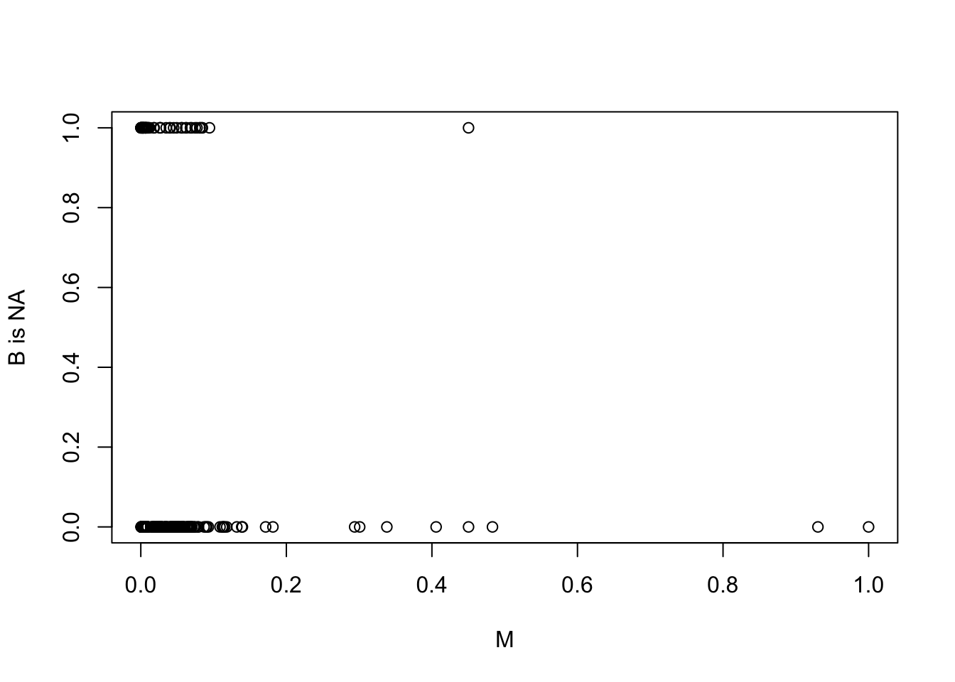 Looks like the missing brain values are almost all for small bodied species. This implies at least a MAR (dog eats students’ homework) mechanism. Let’s try a DAG to express it:
library(dagitty)
hw10.2.1.dag <- dagitty('dag{
M -> R_B -> "B*" <- B
M -> B }')
plot(hw10.2.1.dag)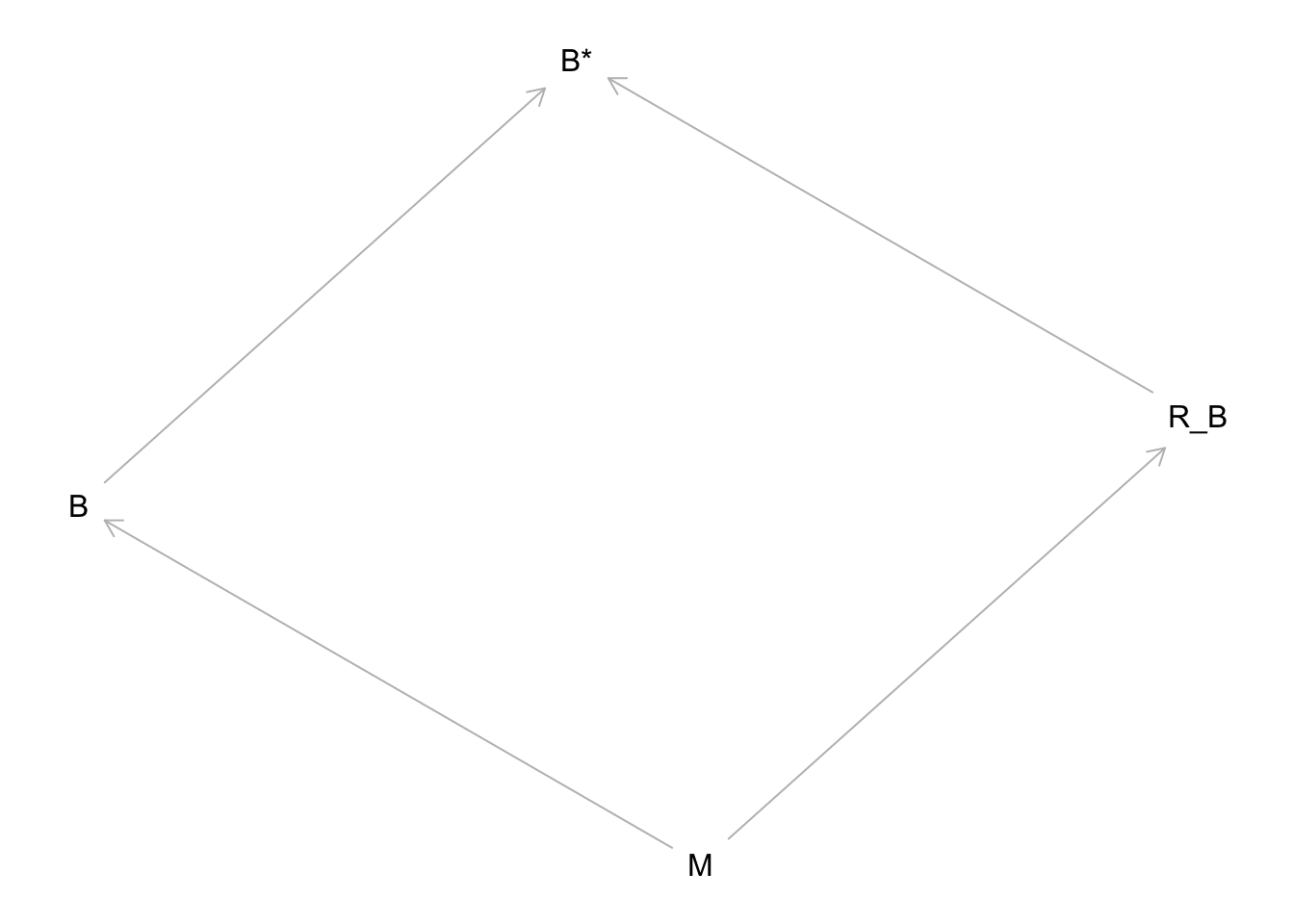 M here is body mass, B (unobserved) is brain size, R_B is the missingness mechanism, and B* is the observed brain sizes (with missing values). The arrow from M to R_B indicates that body size influences missingness. In this case, it would imply that small body size makes a missing brain value more likely.
2.2 impute missing values for brain size
Now let’s do some imputation. Remember that the model for imputation is really no different than an ordinary model. It just needs a prior for any variable with missing values. In this case, the missing values are in the outcome, so the likelihood is the prior we need. So the model doesn’t change at all.
2.2 rethinking
In ulam:
dat_list <- list(
B = B,
M=M)


m2.2 <- ulam( alist(
B ~ dlnorm( mu , sigma ),
mu <- a + b*log(M),
a ~ normal(0,1),
b ~ normal(0,1),
sigma ~ exponential(1) ),
data=dat_list , chains=4 , cores=4 , start=list( B_impute = rep(0.5,56) ) )
ulam figures out how to do the imputation. But an equivalent model that is more explicit would be:
m2.2b <- ulam( alist(
B_merge ~ dlnorm( mu , sigma ),
mu <- a + b*log(M),
B_merge <- merge_missing( B , B_impute ),
a ~ normal(0,1),
b ~ normal(0,1),
sigma ~ exponential(1) ),
data=dat_list , chains=4 , cores=4 , start=list( B_impute = rep(0.5,56) ) )
## Warning: There were 1 divergent transitions after warmup. See
## http://mc-stan.org/misc/warnings.html#divergent-transitions-after-warmup
## to find out why this is a problem and how to eliminate them.## Warning: Examine the pairs() plot to diagnose sampling problems precis( m2.2b )## mean sd 5.5% 94.5% n_eff Rhat4
## a 0.4273296 0.05674211 0.3338733 0.5155636 1009.783 1.004004
## b 0.7832613 0.01371273 0.7606915 0.8046014 1050.283 1.003919
## sigma 0.2936007 0.01576015 0.2695656 0.3203591 1107.455 0.999910It’s a little more obvious now what ulam is doing. It constructs the merged vector of observed and imputed values, B_merge, and then uses that merged vector as the outcome. The outcome distribution at the top of the model is the prior for each B_impute parameter. That prior is adaptive—it has parameters inside it. Hence, shrinkage happens.
2.2 INLA
d2.i <- d %>%
  #only cases with complete body masses
  filter(!is.na(body)) %>%
  mutate(M = body / max(body),
         B= brain / max(brain, na.rm=TRUE),
         logM= log(M))

m2.2.i <- inla(B ~ logM, family ="lognormal", data=d2.i,
               control.fixed = list(
        mean= 0,
        prec= 1,
        mean.intercept= 0,
        prec.intercept= 1),
        control.predictor=list(compute=TRUE)
               )
summary(m2.2.i )
##
## Call:
## c("inla(formula = B ~ logM, family = \"lognormal\", data = d2.i,
## control.predictor = list(compute = TRUE), ", " control.fixed =
## list(mean = 0, prec = 1, mean.intercept = 0, ", " prec.intercept =
## 1))")
## Time used:
## Pre = 1.26, Running = 0.177, Post = 0.2, Total = 1.64
## Fixed effects:
## mean sd 0.025quant 0.5quant 0.975quant mode kld
## (Intercept) 0.427 0.058 0.313 0.427 0.541 0.427 0
## logM 0.783 0.014 0.756 0.783 0.811 0.783 0
##
## Model hyperparameters:
## mean sd 0.025quant 0.5quant
## Precision for the lognormal observations 11.91 1.25 9.60 11.87
## 0.975quant mode
## Precision for the lognormal observations 14.48 11.78
##
## Expected number of effective parameters(stdev): 2.01(0.002)
## Number of equivalent replicates : 90.56
##
## Marginal log-Likelihood: 420.27
## Posterior marginals for the linear predictor and
## the fitted values are computed2.3 compare to the analysis with complete cases
2.3 rethinking
cc2 <- complete.cases( B )
dat_list2 <- list( B = B[cc2],
M = M[cc2] )
m2.3 <- ulam( alist(
B ~ dlnorm( mu , sigma ),
mu <- a + b*log(M),
a ~ normal(0,1),
b ~ normal(0,1),
sigma ~ exponential(1) ),
data=dat_list2 , chains=4 , cores=4 )

precis( m2.3 )
## mean sd 5.5% 94.5% n_eff Rhat4
## a 0.4273367 0.05851702 0.3376391 0.5199382 517.6862 1.009379
## b 0.7832547 0.01406416 0.7618372 0.8058403 550.7742 1.010300
## sigma 0.2928598 0.01561973 0.2688230 0.3181607 850.0766 1.001185Really no difference from before.
2.3 INLA
d3.i <- d2.i %>%
  filter(!is.na(brain))

m2.3.i <- inla(B ~ logM, family ="lognormal", data=d3.i,
               control.fixed = list(
        mean= 0,
        prec= 1,
        mean.intercept= 0,
        prec.intercept= 1),
        control.compute = list(config= TRUE),
        control.predictor=list(compute=TRUE)
               )
summary(m2.3.i )
##
## Call:
## c("inla(formula = B ~ logM, family = \"lognormal\", data = d3.i,
## control.compute = list(config = TRUE), ", " control.predictor =
## list(compute = TRUE), control.fixed = list(mean = 0, ", " prec = 1,
## mean.intercept = 0, prec.intercept = 1))")
## Time used:
## Pre = 1.22, Running = 0.164, Post = 0.205, Total = 1.59
## Fixed effects:
## mean sd 0.025quant 0.5quant 0.975quant mode kld
## (Intercept) 0.427 0.058 0.313 0.427 0.541 0.427 0
## logM 0.783 0.014 0.756 0.783 0.811 0.783 0
##
## Model hyperparameters:
## mean sd 0.025quant 0.5quant
## Precision for the lognormal observations 11.91 1.25 9.60 11.87
## 0.975quant mode
## Precision for the lognormal observations 14.48 11.78
##
## Expected number of effective parameters(stdev): 2.01(0.002)
## Number of equivalent replicates : 90.56
##
## Marginal log-Likelihood: 420.27
## Posterior marginals for the linear predictor and
## the fitted values are computed2.4 plot the imputed brain sizes together with the observed values.
2.4 rethinking
library(rethinking)
post <- rethinking::extract.samples(m2.2)
Bi <- apply( post$B_impute , 2 , mean )
miss_idx <- which( is.na(B) )
plot( M[-miss_idx] , B[-miss_idx] , col=rangi2 , pch=16 , xlab="body mass M" , ylab="brain size B" )
points( M[miss_idx] , Bi )
Bi_ci <- apply( post$B_impute , 2 , PI , 0.5 )
for ( i in 1:length(Bi) ) lines( rep(M[miss_idx][i],2) , Bi_ci[,i] )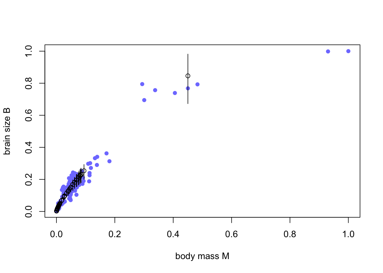
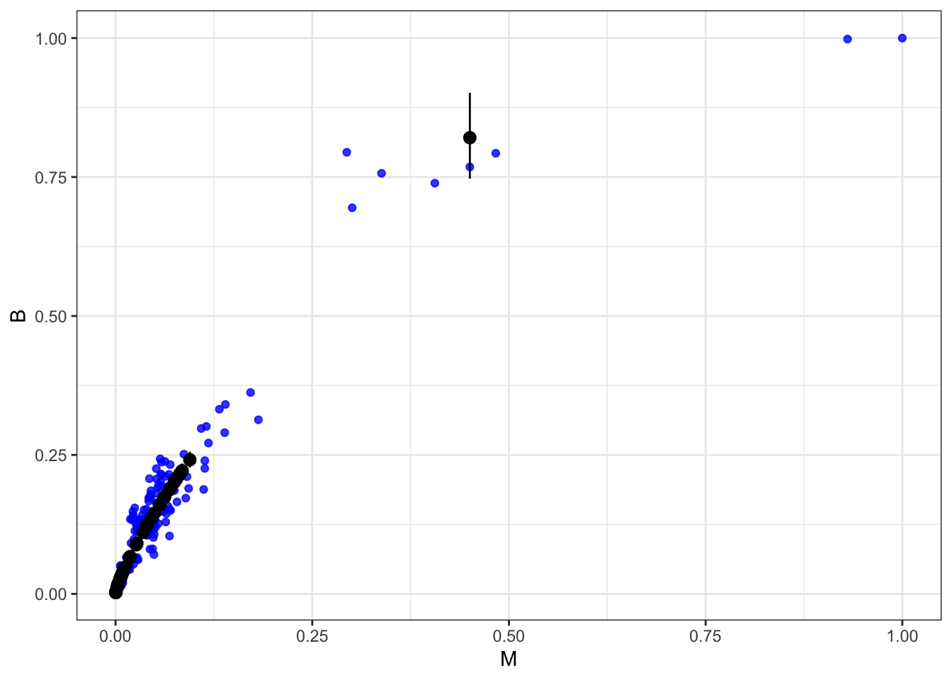
Black open points are the imputed values, with 50% compatibility intervals. Imputation hasn’t done much, apparently because all but one of the missing values are in a very dense region of the body size range. So almost no information was lost—the missing info is redundant.
2.4 INLA
#indices of the weights with missing values of brain
d2.i.na <- which(is.na(d2.i$B))

#cases with response data
d2.i.cc <- d2.i %>%
  filter(!is.na(brain))

#cases with no response data
d2.i.nobrain <- d2.i %>%
  filter(is.na(brain))

#imputed values of the response variable in the response scale exp(brain)
Bi.i <- exp(m2.2.i$summary.fitted.values[d2.i.na,])

#imputed values df

d2.i.imp <- bind_cols(d2.i.nobrain, Bi.i) %>%
  rename("LCI"= "0.025quant", "UCI"= "0.975quant")


m2.2.i.plot <- ggplot() +
  geom_point(data= d2.i.cc, aes(M,B), color= "blue", alpha= 0.8)+
  geom_pointrange(data= d2.i.imp , aes(x= M,  y= mean, ymin= LCI, ymax= UCI))+
  theme_bw()

m2.2.i.plot 