Statistical Rethinking 2nd edition Homework 6 in INLA
library(tidyverse)
library(rethinking)
library(dagitty)
library(INLA)
library(knitr)
library(stringr)
Intro to link functions from Statistical Rethinking 2nd edition Chapter.10
Logit link:
The logit link maps a parameter that is defined as a probability mass, and therefore constrained to lie between zero and one, onto a linear model that can take on any real value. This link is extremely common when working with binomial GLMs. In the context of a model definition, it looks like this:
yi ∼ Binomial(n, pi)
logit(pi) = α + βxi
And the logit function itself is defined as the log-odds:
logit(pi) = log (pi/(1 − pi))
The “odds” of an event are just the probability it happens divided by the probability it does not happen. So really all that is being stated here is:
log (pi/(1 − pi)) = α + βxi
So to figure out the definition of pi implied here, just do a little algebra and solve the above equation for pi:
pi = exp(α + βxi) / 1 + exp(α + βxi)
The above function is usually called the logistic. In this context, it is also commonly called the inverse-logit, because it inverts the logit transform.
No longer does a unit change in a predictor variable produce a constant change in the mean of the outcome variable. Instead, a unit change in xi may produce a larger or smaller change in the probability pi, depending upon how far from zero the log-odds are. For example, in Figure 10.7, when x = 0 the linear model has a value of zero on the log-odds scale. A half- unit increase in x results in about a 0.25 increase in probability. But each addition half-unit will produce less and less of an increase in probability, until any increase is vanishingly small.
The key lesson for now is just that no regression coefficient, such as β, from a GLM ever produces a constant change on the outcome scale. Recall that we defined interaction (Chapter 7) as a situation in which the effect of a predictor depends upon the value of another predictor. Well now every predictor essentially interacts with itself, because the impact of a change in a predictor depends upon the value of the predictor before the change. More generally, every predic- tor variable effectively interacts with every other predictor variable, whether you explicitly model them as interactions or not. This fact makes the visualization of counter-factual pre- dictions even more important for understanding what the model is telling you.
Log link:
This link function maps a parameter that is defined over only positive real values onto a linear model. For example, suppose we want to model the standard deviation σ of a Gaussian distribution so it is a function of a predictor variable x. The parameter σ must be positive, because a standard deviation cannot be negative nor can it be zero. The model might look like:
yi ∼ Normal(μ, σi)
log(σi) = α + βxi
In this model, the mean μ is constant, but the standard deviation scales with the value xi. A log link is both conventional and useful in this situation. It prevents σ from taking on a negative value. What the log link effectively assumes is that the parameter’s value is the exponentiation of the linear model. Solving log(σi) = α + βxi for σi yields the inverse link:
σi = exp(α + βxi)
Using a log link for a linear model (left) implies an exponential scaling of the outcome with the predictor variable (right). Another way to think of this relationship is to remember that logarithms are magnitudes. An increase of one unit on the log scale means an increase of an order of magnitude on the un- transformed scale. And this fact is reflected in the widening intervals between the horizontal lines in the right-hand plot of Figure 10.8. While using a log link does solve the problem of constraining the parameter to be posi- tive, it may also create a problem when the model is asked to predict well outside the range of data used to fit it. Exponential relationships grow, well, exponentially. Just like a lin- ear model cannot be linear forever, an exponential model cannot be exponential forever. Human height cannot be linearly related to weight forever, because very heavy people stop getting taller and start getting wider. Likewise, the property damage caused by a hurricane may be approximately exponentially related to wind speed for smaller storms. But for very big storms, damage may be capped by the fact that everything gets destroyed.
1. data(NWOGrants) What are the total and indirect causal effects of gender on grant awards
The data in data(NWOGrants) are outcomes for scientific funding applications for the Netherlands Organization for Scientific Research (NWO) from 2010–2012 (see van der Lee and Ellemers doi:10.1073/pnas.1510159112). These data have a very similar structure to the UCBAdmit data discussed in Chapter 11. I want you to consider a similar question: What are the total and indirect causal effects of gender on grant awards? Consider a mediation path (a pipe) through discipline. Draw the corresponding DAG and then use one or more binomial GLMs to answer the question. What is your causal interpretation? If NWO’s goal is to equalize rates of funding between the genders, what type of intervention would be most effective?
The implied DAG is:
hw6.1dag <- dagitty("dag{
                  A <- G
                  A<- D
                  D <- G
                  }")
plot(hw6.1dag)
## Plot coordinates for graph not supplied! Generating coordinates, see ?coordinates for how to set your own.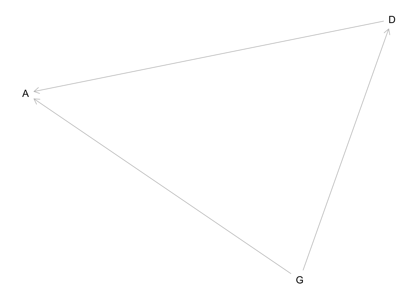
G is gender, D is discipline, and A is award. The direct causal effect of gender is the path G → A. The total effect includes that path and the indirect path G → D → A.
1.a total causal effect of gender
We can estimate the total causal influence (assuming this DAG is correct) with a model that conditions only on gender. I’ll use a N(-1,1) prior for the intercepts, because we know from domain knowledge that less than half of applicants get awards.
1.a rethinking
data(NWOGrants)
d <- NWOGrants
dat_list <- list(
awards = as.integer(d$awards),
apps = as.integer(d$applications),
gid = ifelse( d$gender=="m" , 1L , 2L )
)

m1_total <- ulam(
alist(
awards ~ binomial( apps , p ),
logit(p) <- a[gid],
a[gid] ~ normal(-1,1)
), data=dat_list , chains=4 )
##
## SAMPLING FOR MODEL '81eae820e39db5841689425b0c0bd23c' NOW (CHAIN 1).
## Chain 1:
## Chain 1: Gradient evaluation took 1.8e-05 seconds
## Chain 1: 1000 transitions using 10 leapfrog steps per transition would take 0.18 seconds.
## Chain 1: Adjust your expectations accordingly!
## Chain 1:
## Chain 1:
## Chain 1: Iteration: 1 / 1000 [ 0%] (Warmup)
## Chain 1: Iteration: 100 / 1000 [ 10%] (Warmup)
## Chain 1: Iteration: 200 / 1000 [ 20%] (Warmup)
## Chain 1: Iteration: 300 / 1000 [ 30%] (Warmup)
## Chain 1: Iteration: 400 / 1000 [ 40%] (Warmup)
## Chain 1: Iteration: 500 / 1000 [ 50%] (Warmup)
## Chain 1: Iteration: 501 / 1000 [ 50%] (Sampling)
## Chain 1: Iteration: 600 / 1000 [ 60%] (Sampling)
## Chain 1: Iteration: 700 / 1000 [ 70%] (Sampling)
## Chain 1: Iteration: 800 / 1000 [ 80%] (Sampling)
## Chain 1: Iteration: 900 / 1000 [ 90%] (Sampling)
## Chain 1: Iteration: 1000 / 1000 [100%] (Sampling)
## Chain 1:
## Chain 1: Elapsed Time: 0.010388 seconds (Warm-up)
## Chain 1: 0.009048 seconds (Sampling)
## Chain 1: 0.019436 seconds (Total)
## Chain 1:
##
## SAMPLING FOR MODEL '81eae820e39db5841689425b0c0bd23c' NOW (CHAIN 2).
## Chain 2:
## Chain 2: Gradient evaluation took 8e-06 seconds
## Chain 2: 1000 transitions using 10 leapfrog steps per transition would take 0.08 seconds.
## Chain 2: Adjust your expectations accordingly!
## Chain 2:
## Chain 2:
## Chain 2: Iteration: 1 / 1000 [ 0%] (Warmup)
## Chain 2: Iteration: 100 / 1000 [ 10%] (Warmup)
## Chain 2: Iteration: 200 / 1000 [ 20%] (Warmup)
## Chain 2: Iteration: 300 / 1000 [ 30%] (Warmup)
## Chain 2: Iteration: 400 / 1000 [ 40%] (Warmup)
## Chain 2: Iteration: 500 / 1000 [ 50%] (Warmup)
## Chain 2: Iteration: 501 / 1000 [ 50%] (Sampling)
## Chain 2: Iteration: 600 / 1000 [ 60%] (Sampling)
## Chain 2: Iteration: 700 / 1000 [ 70%] (Sampling)
## Chain 2: Iteration: 800 / 1000 [ 80%] (Sampling)
## Chain 2: Iteration: 900 / 1000 [ 90%] (Sampling)
## Chain 2: Iteration: 1000 / 1000 [100%] (Sampling)
## Chain 2:
## Chain 2: Elapsed Time: 0.010771 seconds (Warm-up)
## Chain 2: 0.010001 seconds (Sampling)
## Chain 2: 0.020772 seconds (Total)
## Chain 2:
##
## SAMPLING FOR MODEL '81eae820e39db5841689425b0c0bd23c' NOW (CHAIN 3).
## Chain 3:
## Chain 3: Gradient evaluation took 1.1e-05 seconds
## Chain 3: 1000 transitions using 10 leapfrog steps per transition would take 0.11 seconds.
## Chain 3: Adjust your expectations accordingly!
## Chain 3:
## Chain 3:
## Chain 3: Iteration: 1 / 1000 [ 0%] (Warmup)
## Chain 3: Iteration: 100 / 1000 [ 10%] (Warmup)
## Chain 3: Iteration: 200 / 1000 [ 20%] (Warmup)
## Chain 3: Iteration: 300 / 1000 [ 30%] (Warmup)
## Chain 3: Iteration: 400 / 1000 [ 40%] (Warmup)
## Chain 3: Iteration: 500 / 1000 [ 50%] (Warmup)
## Chain 3: Iteration: 501 / 1000 [ 50%] (Sampling)
## Chain 3: Iteration: 600 / 1000 [ 60%] (Sampling)
## Chain 3: Iteration: 700 / 1000 [ 70%] (Sampling)
## Chain 3: Iteration: 800 / 1000 [ 80%] (Sampling)
## Chain 3: Iteration: 900 / 1000 [ 90%] (Sampling)
## Chain 3: Iteration: 1000 / 1000 [100%] (Sampling)
## Chain 3:
## Chain 3: Elapsed Time: 0.00957 seconds (Warm-up)
## Chain 3: 0.010369 seconds (Sampling)
## Chain 3: 0.019939 seconds (Total)
## Chain 3:
##
## SAMPLING FOR MODEL '81eae820e39db5841689425b0c0bd23c' NOW (CHAIN 4).
## Chain 4:
## Chain 4: Gradient evaluation took 8e-06 seconds
## Chain 4: 1000 transitions using 10 leapfrog steps per transition would take 0.08 seconds.
## Chain 4: Adjust your expectations accordingly!
## Chain 4:
## Chain 4:
## Chain 4: Iteration: 1 / 1000 [ 0%] (Warmup)
## Chain 4: Iteration: 100 / 1000 [ 10%] (Warmup)
## Chain 4: Iteration: 200 / 1000 [ 20%] (Warmup)
## Chain 4: Iteration: 300 / 1000 [ 30%] (Warmup)
## Chain 4: Iteration: 400 / 1000 [ 40%] (Warmup)
## Chain 4: Iteration: 500 / 1000 [ 50%] (Warmup)
## Chain 4: Iteration: 501 / 1000 [ 50%] (Sampling)
## Chain 4: Iteration: 600 / 1000 [ 60%] (Sampling)
## Chain 4: Iteration: 700 / 1000 [ 70%] (Sampling)
## Chain 4: Iteration: 800 / 1000 [ 80%] (Sampling)
## Chain 4: Iteration: 900 / 1000 [ 90%] (Sampling)
## Chain 4: Iteration: 1000 / 1000 [100%] (Sampling)
## Chain 4:
## Chain 4: Elapsed Time: 0.012404 seconds (Warm-up)
## Chain 4: 0.009471 seconds (Sampling)
## Chain 4: 0.021875 seconds (Total)
## Chain 4:precis(m1_total,2)## mean sd 5.5% 94.5% n_eff Rhat4
## a[1] -1.534215 0.06419862 -1.636220 -1.433608 1270.353 1.001674
## a[2] -1.739403 0.08338316 -1.876282 -1.605273 1458.263 1.002103Gender 1 here is male and 2 is female. So males have higher rates of award, on average. How big is the difference? Let’s look at the contrast on absolute (penguin) scale:
post <- extract.samples(m1_total)
diff <- inv_logit( post$a[,1] ) - inv_logit(post$a[,2])
precis( list( diff=diff ) )
## mean sd 5.5% 94.5% histogram
## diff 0.02787365 0.01386206 0.005582129 0.05019898 ▁▁▂▅▇▇▃▁▁So a small 3% difference on average. Still, with such low funding rates (in some disciplines), 3% is a big advantage.
1.a inla
data(NWOGrants)
d <- NWOGrants

d1.i <- d %>%
  mutate(g_val= 1,
         d= paste("d", as.integer(discipline), sep = "."),
         d_val= 1) %>%
  spread(gender, g_val) %>%
  spread(d, d_val)

# number of trials is d1.i$applications

m1a.i <- inla(awards ~ -1 + m + f , data= d1.i, family = "binomial",
              Ntrials = applications,
              control.family = list(control.link=list(model="logit")),
              control.fixed = list(
        mean= -1,
        prec= 1),
              control.predictor=list(link=1, compute=T),
              control.compute=list(config=T))
summary(m1a.i)
##
## Call:
## c("inla(formula = awards ~ -1 + m + f, family = \"binomial\", data =
## d1.i, ", " Ntrials = applications, control.compute = list(config = T),
## ", " control.predictor = list(link = 1, compute = T), control.family =
## list(control.link = list(model = \"logit\")), ", " control.fixed =
## list(mean = -1, prec = 1))")
## Time used:
## Pre = 1.55, Running = 0.15, Post = 0.159, Total = 1.86
## Fixed effects:
## mean sd 0.025quant 0.5quant 0.975quant mode kld
## m -1.532 0.065 -1.660 -1.531 -1.407 -1.530 0
## f -1.738 0.081 -1.899 -1.737 -1.581 -1.735 0
##
## Expected number of effective parameters(stdev): 1.99(0.00)
## Number of equivalent replicates : 9.04
##
## Marginal log-Likelihood: -66.79
## Posterior marginals for the linear predictor and
## the fitted values are computed#computed in the outcome scale
m1a.i$summary.fitted.values## mean sd 0.025quant 0.5quant 0.975quant
## fitted.Predictor.01 0.1499131 0.010317651 0.1301956 0.1497340 0.1706421
## fitted.Predictor.02 0.1779058 0.009440579 0.1597389 0.1777855 0.1967474
## fitted.Predictor.03 0.1499091 0.010316723 0.1301934 0.1497302 0.1706361
## fitted.Predictor.04 0.1779085 0.009440072 0.1597425 0.1777883 0.1967490
## fitted.Predictor.05 0.1499154 0.010316754 0.1301995 0.1497365 0.1706424
## fitted.Predictor.06 0.1778922 0.009438767 0.1597286 0.1777720 0.1967300
## fitted.Predictor.07 0.1499140 0.010317386 0.1301970 0.1497350 0.1706424
## fitted.Predictor.08 0.1778933 0.009439873 0.1597277 0.1777730 0.1967335
## fitted.Predictor.09 0.1779015 0.009439025 0.1597374 0.1777813 0.1967398
## fitted.Predictor.10 0.1499020 0.010315236 0.1301889 0.1497232 0.1706259
## fitted.Predictor.11 0.1499123 0.010317606 0.1301949 0.1497333 0.1706412
## fitted.Predictor.12 0.1779011 0.009439942 0.1597354 0.1777808 0.1967414
## fitted.Predictor.13 0.1499103 0.010317738 0.1301928 0.1497313 0.1706396
## fitted.Predictor.14 0.1779047 0.009440672 0.1597377 0.1777845 0.1967466
## fitted.Predictor.15 0.1498987 0.010313838 0.1301880 0.1497199 0.1706195
## fitted.Predictor.16 0.1778898 0.009437012 0.1597294 0.1777697 0.1967239
## fitted.Predictor.17 0.1499127 0.010317445 0.1301957 0.1497337 0.1706413
## fitted.Predictor.18 0.1778960 0.009439275 0.1597316 0.1777758 0.1967349
## mode
## fitted.Predictor.01 0.1493748
## fitted.Predictor.02 0.1775440
## fitted.Predictor.03 0.1493710
## fitted.Predictor.04 0.1775469
## fitted.Predictor.05 0.1493774
## fitted.Predictor.06 0.1775307
## fitted.Predictor.07 0.1493758
## fitted.Predictor.08 0.1775316
## fitted.Predictor.09 0.1775400
## fitted.Predictor.10 0.1493642
## fitted.Predictor.11 0.1493740
## fitted.Predictor.12 0.1775394
## fitted.Predictor.13 0.1493720
## fitted.Predictor.14 0.1775430
## fitted.Predictor.15 0.1493611
## fitted.Predictor.16 0.1775286
## fitted.Predictor.17 0.1493745
## fitted.Predictor.18 0.1775345#contrast between male and female
n.samples = 1000
#pi = exp(α + βxi) / 1 + exp(α + βxi)
inverse_logit <- function (x){
p <- 1/(1 + exp(-x))
p <- ifelse(x == Inf, 1, p)
p }
m1a.i.samples = inla.posterior.sample(n.samples, result = m1a.i)
m1a.i.contrast1 <- inla.posterior.sample.eval(function(...) {
inverse_logit(m) -
inverse_logit(f)
},
m1a.i.samples)
summary(as.vector(m1a.i.contrast1))## Min. 1st Qu. Median Mean 3rd Qu. Max.
## -0.01821 0.01887 0.02837 0.02807 0.03775 0.073591.b direct effect of gender
Now for the direct influence of gender, we condition on discipline as well:
1.b rethinking
dat_list$disc <- as.integer(d$discipline)

m1_direct <- ulam(
alist(
awards ~ binomial( apps , p ),
logit(p) <- a[gid] + d[disc],
a[gid] ~ normal(-1,1),
d[disc] ~ normal(0,1)
),
data=dat_list , chains=4 , cores=4 , iter=3000 )

precis(m1_direct,2)
## mean sd 5.5% 94.5% n_eff Rhat4
## a[1] -1.360704267 0.3065706 -1.8587853 -0.86263022 586.7668 1.003143
## a[2] -1.501544865 0.3128893 -2.0028811 -0.99711205 611.3386 1.002769
## d[1] 0.342608770 0.3559347 -0.2262837 0.90898810 768.4841 1.002029
## d[2] 0.020314490 0.3303936 -0.5055576 0.55236030 691.4877 1.003546
## d[3] -0.213318382 0.3260893 -0.7367684 0.31247347 705.1018 1.002649
## d[4] -0.252491812 0.3552531 -0.8202482 0.31097573 820.0334 1.001536
## d[5] -0.315338973 0.3256869 -0.8271814 0.21124122 644.0385 1.002919
## d[6] 0.001451087 0.3458133 -0.5616136 0.55976413 812.7953 1.001885
## d[7] 0.312613425 0.3807893 -0.2961343 0.92932199 977.8970 1.000619
## d[8] -0.435891933 0.3182044 -0.9471851 0.09015475 592.5001 1.002909
## d[9] -0.190623298 0.3346838 -0.7231056 0.35118272 708.5796 1.002368Those chains didn’t sample very efficiently. This likely because the model is over- parameterized—it has more parameters than absolutely necessary. This doesn’t break it. It just makes the sampling less efficient. Anyway, now we can compute the gender difference again. On the relative scale:
post <- extract.samples(m1_direct)
diff_a <- post$a[,1] - post$a[,2]
precis( list( diff_a=diff_a ) )
## mean sd 5.5% 94.5% histogram
## diff_a 0.1408406 0.1083074 -0.0312027 0.3181228 ▁▁▂▅▇▅▁▁▁Still an advantage for the males, but reduced and overlapping zero a bit. To see this difference on the absolute scale, we need to account for the base rates in each discipline as well. If you look at the postcheck(m1_direct) display, you’ll see the predictive difference is very small. There are also several disciplines that reverse the advantage. If there is a direct influence of gender here, it is small, much smaller than before we accounted for discipline. Why? Because again the disciplines have different funding rates and women apply more to the disciplines with lower funding rates. But it would be hasty, I think, to conclude there are no other influences. There are after all lots of unmeasured confounds…
postcheck(m1_direct)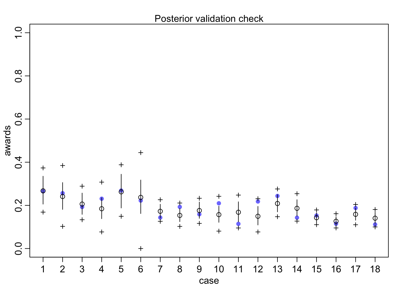
1.b inla
data(NWOGrants)
d <- NWOGrants

d1.i <- d %>%
  mutate(g_val= 1,
         d= paste("d", as.integer(discipline), sep = "."),
         d_val= 1) %>%
  spread(gender, g_val) %>%
  spread(d, d_val)

# number of trials is d1.i$applications

d_names <- paste("d", 1:9, sep = ".")

m1b.i <- inla(awards ~ -1 + m + f + d.1+d.2+d.3+d.4+d.5+d.6+d.7+d.8+d.9, data= d1.i, family = "binomial",
              Ntrials = applications,
              control.family = list(control.link=list(model="logit")),
              control.fixed = list(
        mean= list(m=-1,f=-1, d.1=0, d.2=0, d.3=0, d.4=0,d.5=0,d.6=0,d.7=0,d.8=0,d.9),
        prec= 1),
              control.predictor=list(link=1, compute=T),
              control.compute=list(config=T))
summary(m1b.i)
##
## Call:
## c("inla(formula = awards ~ -1 + m + f + d.1 + d.2 + d.3 + d.4 + ", "
## d.5 + d.6 + d.7 + d.8 + d.9, family = \"binomial\", data = d1.i, ", "
## Ntrials = applications, control.compute = list(config = T), ", "
## control.predictor = list(link = 1, compute = T), control.family =
## list(control.link = list(model = \"logit\")), ", " control.fixed =
## list(mean = list(m = -1, f = -1, d.1 = 0, ", " d.2 = 0, d.3 = 0, d.4 =
## 0, d.5 = 0, d.6 = 0, d.7 = 0, ", " d.8 = 0, d.9), prec = 1))")
## Time used:
## Pre = 1.98, Running = 0.184, Post = 0.265, Total = 2.43
## Fixed effects:
## mean sd 0.025quant 0.5quant 0.975quant mode kld
## m -1.348 0.308 -1.953 -1.348 -0.745 -1.348 0
## f -1.488 0.313 -2.102 -1.488 -0.875 -1.488 0
## d.1 0.336 0.356 -0.365 0.337 1.033 0.339 0
## d.2 0.008 0.333 -0.647 0.009 0.661 0.009 0
## d.3 -0.224 0.329 -0.870 -0.223 0.420 -0.223 0
## d.4 -0.263 0.354 -0.961 -0.262 0.428 -0.259 0
## d.5 -0.328 0.326 -0.967 -0.327 0.310 -0.327 0
## d.6 -0.008 0.349 -0.696 -0.007 0.674 -0.006 0
## d.7 0.304 0.383 -0.453 0.306 1.050 0.310 0
## d.8 -0.448 0.319 -1.074 -0.447 0.178 -0.447 0
## d.9 -0.196 0.340 -0.866 -0.196 0.469 -0.195 0
##
## Expected number of effective parameters(stdev): 9.75(0.00)
## Number of equivalent replicates : 1.85
##
## Marginal log-Likelihood: -71.14
## Posterior marginals for the linear predictor and
## the fitted values are computed#contrast between male and female
n.samples = 1000
m1b.i.samples = inla.posterior.sample(n.samples, result = m1b.i)
#On the relative scale:
m1b.i.contrast1 <- inla.posterior.sample.eval(function(...) {
m - f
},
m1b.i.samples)
summary(as.vector(m1b.i.contrast1))## Min. 1st Qu. Median Mean 3rd Qu. Max.
## -0.18750 0.06853 0.14537 0.14439 0.21724 0.479842. data(NWOGrants) unobserved confound that influences both choice of discipline and the probability of an award
Suppose that the NWO Grants sample has an unobserved confound that influences both choice of discipline and the probability of an award. One example of such a confound could be the career stage of each applicant. Suppose that in some disciplines, junior scholars apply for most of the grants. In other disciplines, scholars from all career stages compete. As a result, career stage influences discipline as well as the probability of being awarded a grant. Add these influences to your DAG from Problem 1. What happens now when you condition on discipline? Does it provide an un-confounded estimate of the direct path from gender to an award? Why or why not? Justify your answer with the back-door criterion. Hint: This is structurally a lot like the grandparents-parents- children-neighborhoods example from a previous week. If you have trouble thinking this though, try simulating fake data, assuming your DAG is true. Then analyze it using the model from Problem 1. What do you conclude? Is it possible for gender to have a real direct causal influence but for a regression conditioning on both gender and discipline to suggest zero influence?
hw6.2dag <- dagitty("dag{
                  A <- G
                  A<- D
                  D <- G
                  D <- S
                  A <- S
                  }")
plot(hw6.2dag)
## Plot coordinates for graph not supplied! Generating coordinates, see ?coordinates for how to set your own.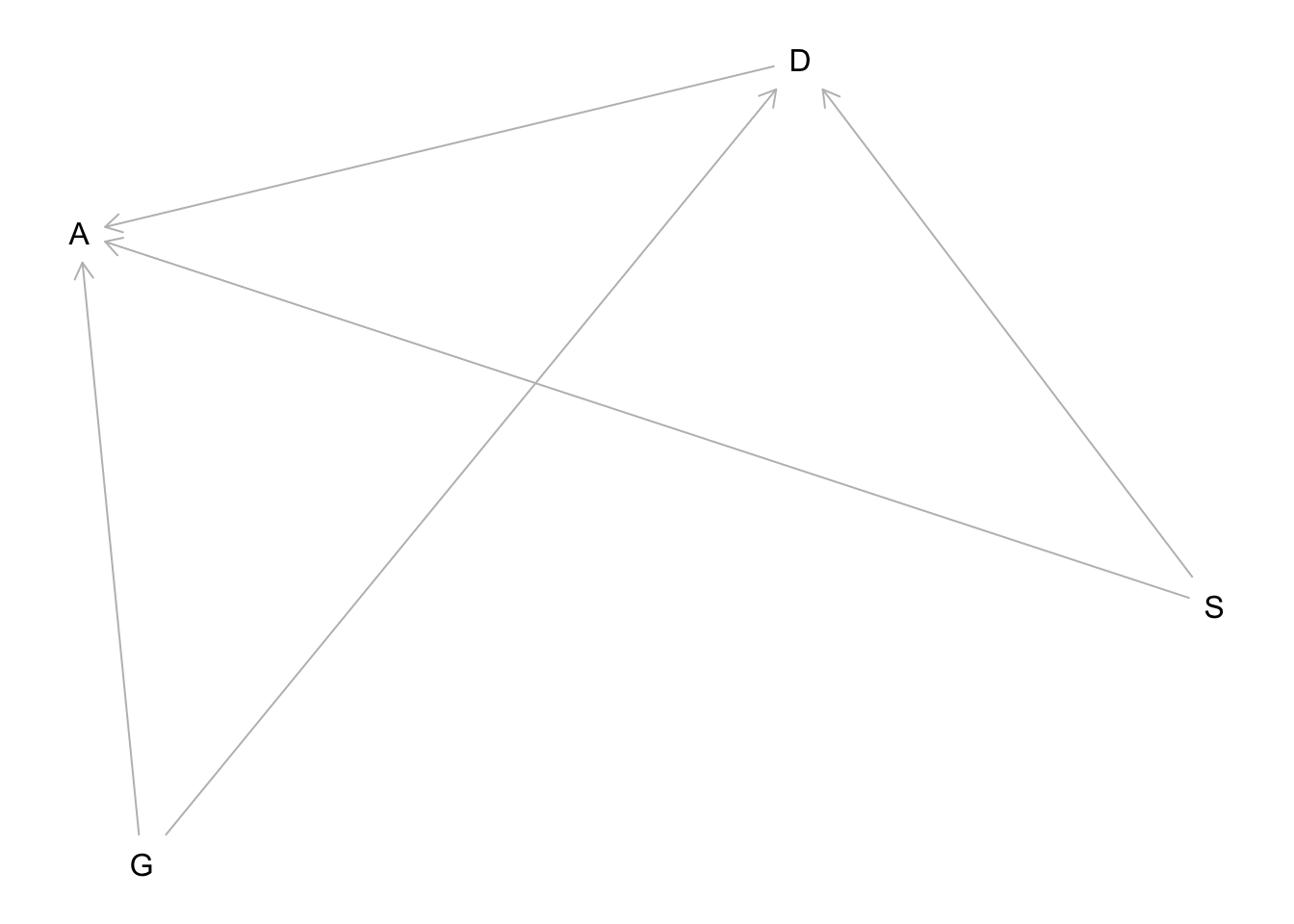
S is stage of career (unobserved). This DAG has the same structure as the grandparents-parents-children-neighborhoods example from earlier in the course. When we condition on discipline D it opens a backdoor path through S to A.
It is not possible here to get an unconfounded estimate of gender on awards.
Here’s a simulation to demonstrate the potential issue: This code simulates 1000 applicants. There are 2 genders (G 0/1), 2 stages of career (S 0/1), and 2 disciplines (D 0/1). Discipline 1 is chosen more by gender 1 and career stage 1. So that could mean more by males and later stage of career. Then awards A have a consistent bias towards gender 1, and discipline 1 has a higher award rate, and stage 1 also a higher award rate. If we analyze these data:
2.a rethinking
set.seed(1913)
N <- 1000
G <- rbern(N)
S <- rbern(N)
D <- rbern( N , p=inv_logit( G + S ) )
A <- rbern( N , p=inv_logit( 0.25*G + D + 2*S - 2 ) )
dat_sim <- list( G=G , D=D , A=A )

m2_sim <- ulam( alist(
A ~ bernoulli(p),
logit(p) <- a + d*D + g*G,
c(a,d,g) ~ normal(0,1)
), data=dat_sim , chains=4 , cores=4 )

precis(m2_sim)
## mean sd 5.5% 94.5% n_eff Rhat4
## g 0.3396301 0.1301321 0.1257989 0.5480141 826.6339 1.003988
## d 1.2227536 0.1588039 0.9707247 1.4763537 731.3829 1.004335
## a -1.0780455 0.1421107 -1.3062138 -0.8520954 729.2983 1.004582The parameter g is the advantage of gender 1. It is smaller than the true advantage and the estimate straddles zero quite a lot, even with 1000 applicants.
2.a INLA
Reference: https://rpubs.com/corey_sparks/431920
set.seed(1913)
N <- 1000
G <- rbern(N)
S <- rbern(N)
D <- rbern( N , p=inv_logit( G + S ) )
A <- rbern( N , p=inv_logit( 0.25*G + D + 2*S - 2 ) )
dat_sim <- list( G=G , D=D , A=A )

m2a.i <- inla(A ~ D+G, data= dat_sim, family = "binomial",
              Ntrials = 1, #Ntrials=1 for bernoulli, logistic regression
              control.family = list(control.link=list(model="logit")),
              control.fixed = list(
        mean= 0,
        prec= 1,
        mean.intercept= 0,
        prec.intercept= 1),
              control.predictor=list(link=1, compute=T),
              control.compute=list(config=T))
summary(m2a.i)
##
## Call:
## c("inla(formula = A ~ D + G, family = \"binomial\", data = dat_sim, ",
## " Ntrials = 1, control.compute = list(config = T), control.predictor =
## list(link = 1, ", " compute = T), control.family = list(control.link =
## list(model = \"logit\")), ", " control.fixed = list(mean = 0, prec = 1,
## mean.intercept = 0, ", " prec.intercept = 1))")
## Time used:
## Pre = 1.39, Running = 0.257, Post = 0.219, Total = 1.87
## Fixed effects:
## mean sd 0.025quant 0.5quant 0.975quant mode kld
## (Intercept) -1.073 0.143 -1.358 -1.072 -0.798 -1.069 0
## D 1.216 0.155 0.914 1.214 1.523 1.212 0
## G 0.345 0.132 0.085 0.345 0.604 0.345 0
##
## Expected number of effective parameters(stdev): 2.94(0.00)
## Number of equivalent replicates : 340.19
##
## Marginal log-Likelihood: -657.91
## Posterior marginals for the linear predictor and
## the fitted values are computedIt is also possible to have no gender influence and infer it by accident. Try these settings: ### 2.b rethinking
set.seed(1913)
N <- 1000
G <- rbern(N)
S <- rbern(N)
D <- rbern( N , p=inv_logit( 2*G - S ) )
A <- rbern( N , p=inv_logit( 0*G + D + S - 2 ) )
dat_sim2 <- list( G=G , D=D , A=A )
m2_sim_2 <- ulam( m2_sim , data=dat_sim2 , chains=4 , cores=4 )

precis(m2_sim_2,2)
## mean sd 5.5% 94.5% n_eff Rhat4
## g 0.2500214 0.1468850 0.007746612 0.4856631 931.1880 0.9999269
## d 0.2719462 0.1543328 0.023773557 0.5164615 962.4796 0.9987312
## a -1.1241445 0.1196152 -1.313980496 -0.9409501 1070.1102 1.0003390Now it looks like gender 1 has a consistent advantage, but in fact there is no advan- tage in the simulation.
2.b INLA
set.seed(1913)
N <- 1000
G <- rbern(N)
S <- rbern(N)
D <- rbern( N , p=inv_logit( 2*G - S ) )
A <- rbern( N , p=inv_logit( 0*G + D + S - 2 ) )
dat_sim2 <- list( G=G , D=D , A=A )

m2b.i <- inla(A ~ D+G, data= dat_sim2, family = "binomial",
              Ntrials = 1, #Ntrials=1 for bernoulli, logistic regression
              control.family = list(control.link=list(model="logit")),
              control.fixed = list(
        mean= 0,
        prec= 1,
        mean.intercept= 0,
        prec.intercept= 1),
              control.predictor=list(link=1, compute=T),
              control.compute=list(config=T))
summary(m2b.i)
##
## Call:
## c("inla(formula = A ~ D + G, family = \"binomial\", data = dat_sim2, ",
## " Ntrials = 1, control.compute = list(config = T), control.predictor =
## list(link = 1, ", " compute = T), control.family = list(control.link =
## list(model = \"logit\")), ", " control.fixed = list(mean = 0, prec = 1,
## mean.intercept = 0, ", " prec.intercept = 1))")
## Time used:
## Pre = 1.28, Running = 0.287, Post = 0.176, Total = 1.74
## Fixed effects:
## mean sd 0.025quant 0.5quant 0.975quant mode kld
## (Intercept) -1.120 0.119 -1.358 -1.119 -0.889 -1.116 0
## D 0.269 0.156 -0.036 0.269 0.576 0.268 0
## G 0.251 0.151 -0.044 0.251 0.548 0.251 0
##
## Expected number of effective parameters(stdev): 2.94(0.00)
## Number of equivalent replicates : 340.13
##
## Marginal log-Likelihood: -616.04
## Posterior marginals for the linear predictor and
## the fitted values are computed3. data(Primates301) brain size is associated with social learning
The data in data(Primates301) were first introduced at the end of Chapter7. In this problem, you will consider how brain size is associated with social learning. There are three parts.
3.1 model the number of observations of social_learning for each species as a function of the log brain size
First, model the number of observations of social_learning for each species as a function of the log brain size. Use a Poisson distribution for the social_learning outcome variable. Interpret the resulting posterior.
Now we first want a model with social learning as the outcome and brain size as a predictor. For this Poisson GLM, I’m going to use a N(0,1) prior on the intercept, since we know the counts should be small.
3.1.a rethinking
library(rethinking)
data(Primates301)
d <- Primates301
d3 <- d[ complete.cases( d$social_learning , d$brain , d$research_effort),]

dat <- list(
soc_learn = d3$social_learning,
log_brain = standardize( log(d3$brain) ), log_effort = log(d3$research_effort)
)

m3_1 <- ulam( alist(
soc_learn ~ poisson( lambda ), log(lambda) <- a + bb*log_brain, a ~ normal(0,1),
bb ~ normal(0,0.5)
), data=dat , chains=4 , cores=4 )
## Warning: Bulk Effective Samples Size (ESS) is too low, indicating posterior means and medians may be unreliable.
## Running the chains for more iterations may help. See
## http://mc-stan.org/misc/warnings.html#bulk-essprecis( m3_1 )## mean sd 5.5% 94.5% n_eff Rhat4
## a -1.18137 0.1197506 -1.375183 -0.9890849 362.9303 1.001218
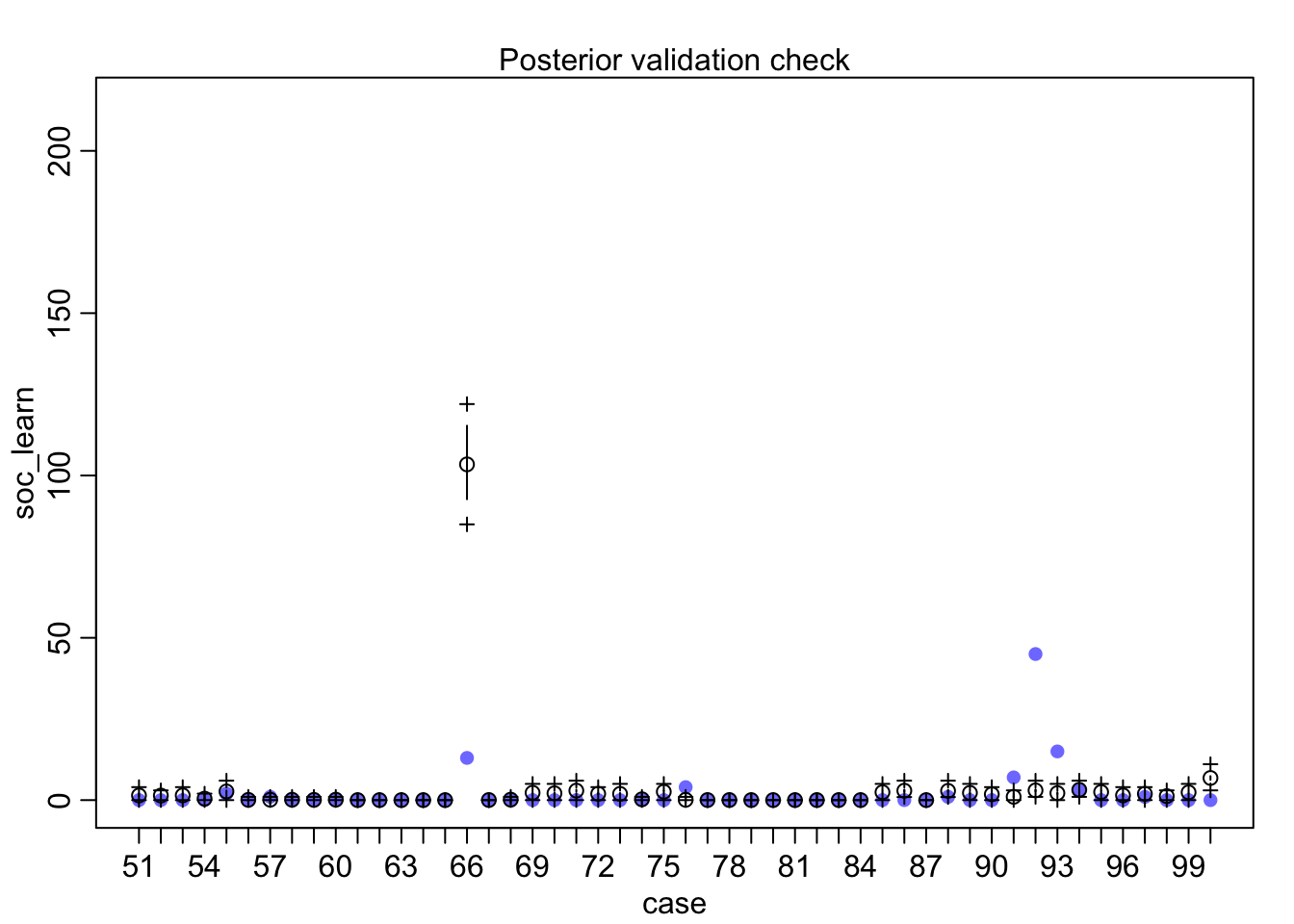
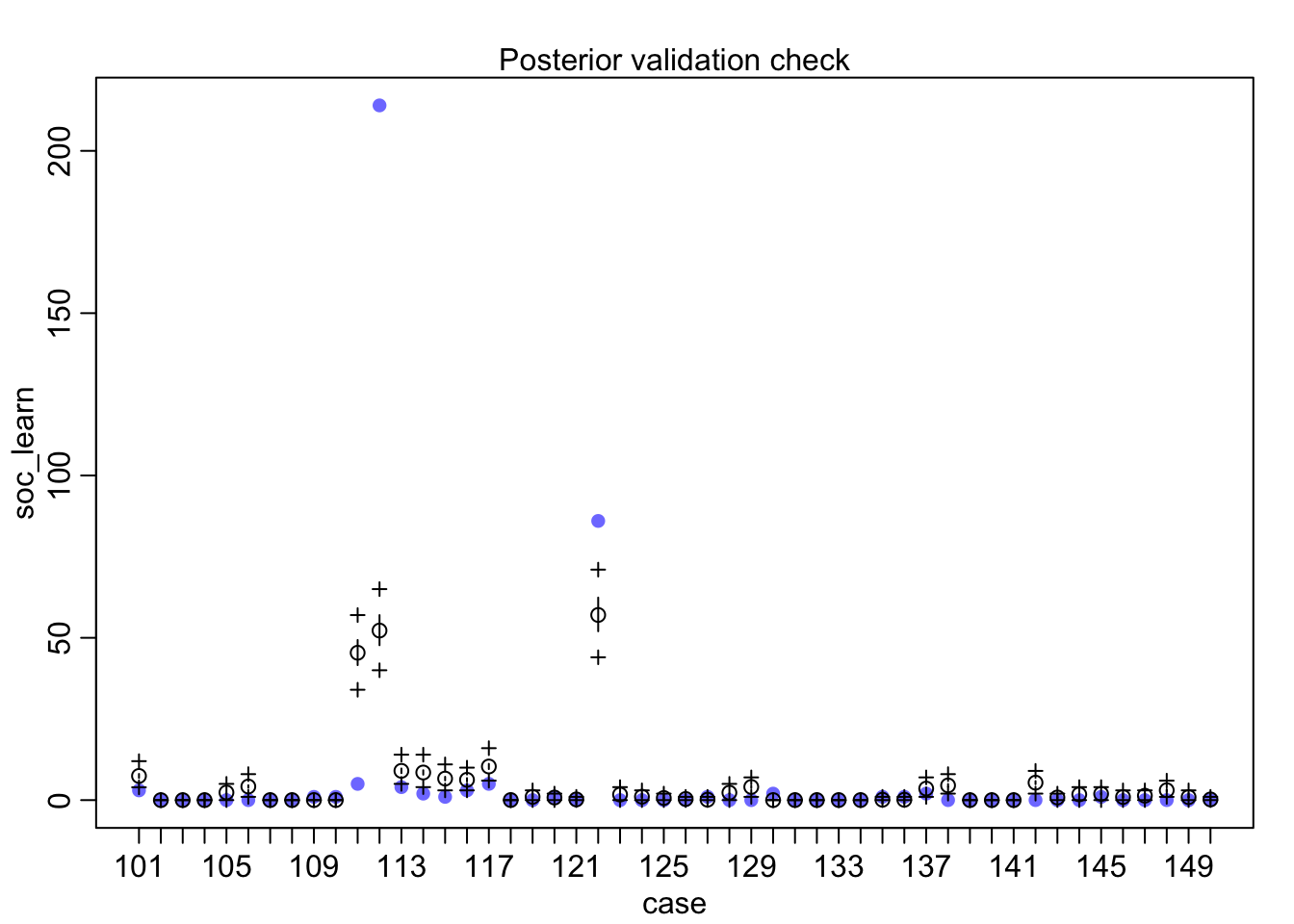
## bb 2.76474 0.0762447 2.644873 2.8864750 380.3295 1.001877postcheck(m3_1,window=50)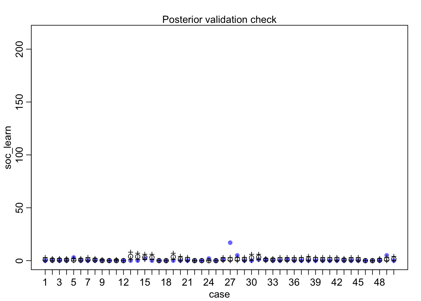
3.1.a INLA
library(rethinking)
data(Primates301)
d <- Primates301
d3.i <- d[ complete.cases( d$social_learning , d$brain , d$research_effort),] %>%
  mutate(soc_learn = social_learning,
log_brain = standardize( log(brain) ),
log_effort = log(research_effort),
case= row_number())

m3.1.i <- inla( soc_learn~ log_brain, family='poisson',
   data=d3.i,
   control.fixed = list(
        mean= 0,
        prec= 1,
        mean.intercept= 0,
        prec.intercept= 1/(0.5^2)),
   control.family=list(link='log'),
   control.predictor=list(link=1, compute=TRUE),
   control.compute=list(dic=TRUE, cpo=TRUE, waic=TRUE))

summary(m3.1.i)
##
## Call:
## c("inla(formula = soc_learn ~ log_brain, family = \"poisson\", data =
## d3.i, ", " control.compute = list(dic = TRUE, cpo = TRUE, waic = TRUE),
## ", " control.predictor = list(link = 1, compute = TRUE), control.family
## = list(link = \"log\"), ", " control.fixed = list(mean = 0, prec = 1,
## mean.intercept = 0, ", " prec.intercept = 1/(0.5^2)))")
## Time used:
## Pre = 1.35, Running = 0.175, Post = 0.169, Total = 1.7
## Fixed effects:
## mean sd 0.025quant 0.5quant 0.975quant mode kld
## (Intercept) -1.190 0.116 -1.421 -1.188 -0.966 -1.185 0
## log_brain 2.778 0.074 2.634 2.778 2.924 2.777 0
##
## Expected number of effective parameters(stdev): 1.94(0.00)
## Number of equivalent replicates : 77.20
##
## Deviance Information Criterion (DIC) ...............: 1237.72
## Deviance Information Criterion (DIC, saturated) ....: 1123.01
## Effective number of parameters .....................: 1.94
##
## Watanabe-Akaike information criterion (WAIC) ...: 1405.31
## Effective number of parameters .................: 138.86
##
## Marginal log-Likelihood: -628.73
## CPO and PIT are computed
##
## Posterior marginals for the linear predictor and
## the fitted values are computedinla postcheck
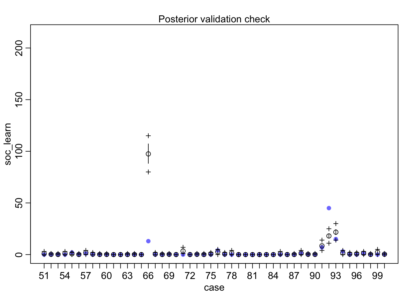
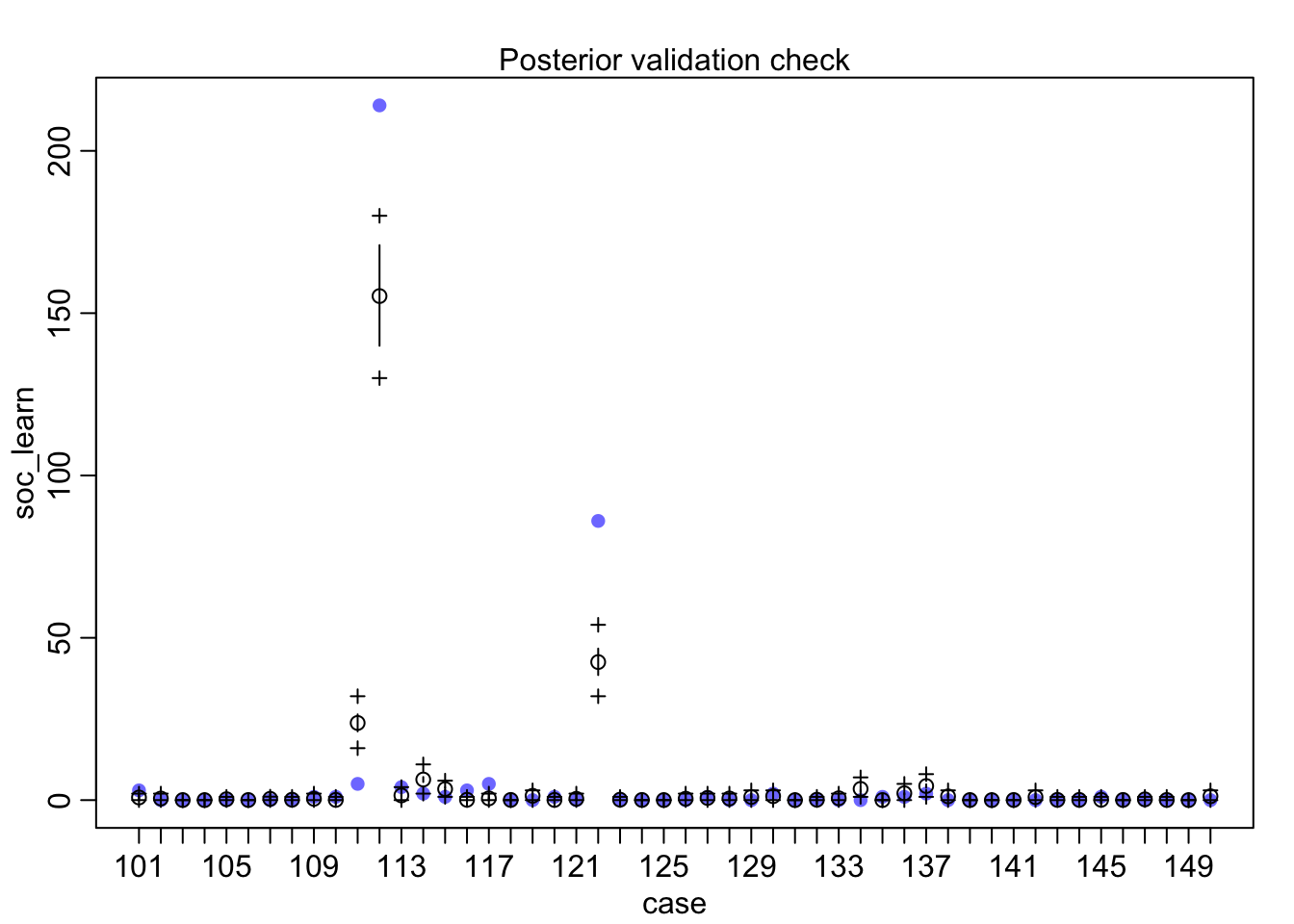
m3.1.i.postcheck <- bind_cols(d3.i[, c("case", "soc_learn")], m3.1.i$summary.fitted.values)

names(m3.1.i.postcheck) <- c("case", "soc_learn", "mean", "sd", "LCI", "MCI",
"UCI", "mode")

m3.1.i.postcheck.plot <- ggplot() +
  geom_point(data= m3.1.i.postcheck, aes(x= case, y= soc_learn), color= "blue", alpha= 0.5)+
  geom_pointrange(data= m3.1.i.postcheck, aes(x= case, y= mean, ymin= LCI, ymax= UCI ), color= "red", alpha= 0.3, size= 0.15)+
  theme_bw()


m3.1.i.postcheck.plot 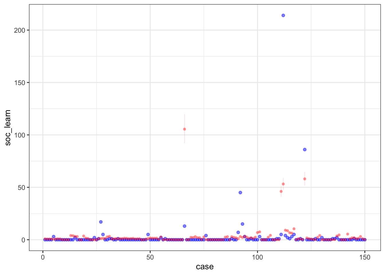
The blue points are the raw data, recall. These are not great posterior predictions. Clearly other factors are in play.
Let’s try the research effort variable now.
3.2 Use the research_effort variable, specifically its logarithm, as an additional predictor variable
Second, some species are studied much more than others. So the number of reported instances of social_learning could be a product of research effort. Use the research_effort variable, specifically its logarithm, as an additional predictor variable. Interpret the coefficient for log research_effort. Does this model disagree with the previous one?
3.2 rethinking
library(rethinking)
data(Primates301)
d <- Primates301
d3 <- d[ complete.cases( d$social_learning , d$brain , d$research_effort),]

dat <- list(
soc_learn = d3$social_learning,
log_brain = standardize( log(d3$brain) ), log_effort = log(d3$research_effort)
)

m3_2 <- ulam( alist(
soc_learn ~ poisson( lambda ),
log(lambda) <- a + be*log_effort + bb*log_brain,
a ~ normal(0,1),
c(bb,be) ~ normal(0,0.5)
), data=dat , chains=4 , cores=4 )
precis( m3_2 )
## mean sd 5.5% 94.5% n_eff Rhat4
## a -5.9639980 0.31815132 -6.5096372 -5.4737698 461.4116 1.002493
## be 1.5312013 0.06703299 1.4275654 1.6432004 409.8507 1.004445
## bb 0.4631976 0.08152311 0.3369609 0.5932976 577.9021 1.005852precis( m3_2)## mean sd 5.5% 94.5% n_eff Rhat4
## a -5.9639980 0.31815132 -6.5096372 -5.4737698 461.4116 1.002493
## be 1.5312013 0.06703299 1.4275654 1.6432004 409.8507 1.004445
## bb 0.4631976 0.08152311 0.3369609 0.5932976 577.9021 1.005852postcheck(m3_2,window=50)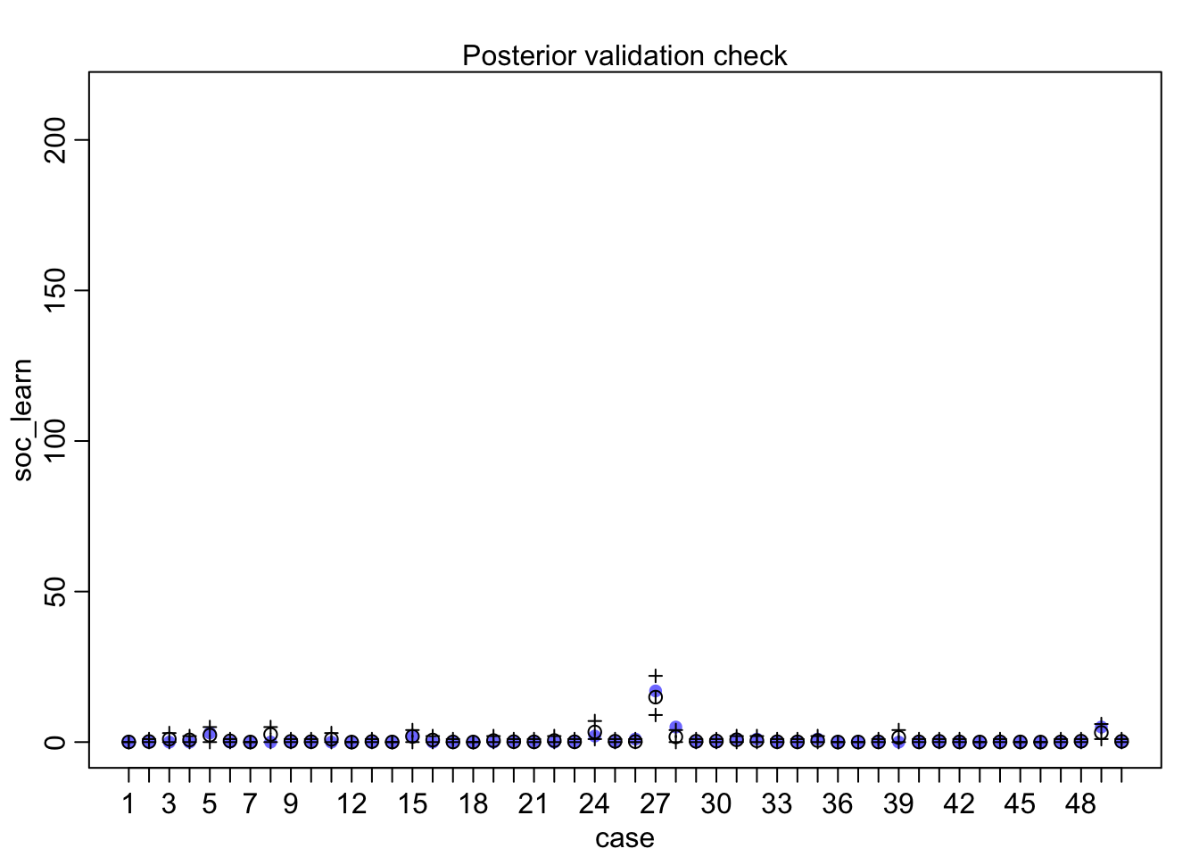
Brain size bb is still positively associated, but much less. Research effort be is strongly associated. To see how these models disagree, let’s use pointwise WAIC to see which cases each predicts well.
3.2 INLA
library(rethinking)
data(Primates301)
d <- Primates301
d3.i <- d[ complete.cases( d$social_learning , d$brain , d$research_effort),] %>%
  mutate(soc_learn = social_learning,
log_brain = standardize( log(brain) ),
log_effort = log(research_effort),
case= row_number())

m3.2.i <- inla( soc_learn~ log_brain + log_effort, family='poisson',
   data=d3.i,
   control.fixed = list(
        mean= 0,
        prec= 1,
        mean.intercept= 0,
        prec.intercept= 1/(0.5^2)),
   control.family=list(link='log'),
   control.predictor=list(link=1, compute=TRUE),
   control.compute=list(dic=TRUE, cpo=TRUE, waic=TRUE))

summary(m3.2.i)
##
## Call:
## c("inla(formula = soc_learn ~ log_brain + log_effort, family =
## \"poisson\", ", " data = d3.i, control.compute = list(dic = TRUE, cpo =
## TRUE, ", " waic = TRUE), control.predictor = list(link = 1, compute =
## TRUE), ", " control.family = list(link = \"log\"), control.fixed =
## list(mean = 0, ", " prec = 1, mean.intercept = 0, prec.intercept =
## 1/(0.5^2)))" )
## Time used:
## Pre = 1.39, Running = 0.202, Post = 0.221, Total = 1.81
## Fixed effects:
## mean sd 0.025quant 0.5quant 0.975quant mode kld
## (Intercept) -4.833 0.239 -5.310 -4.831 -4.372 -4.825 0
## log_brain 0.614 0.080 0.461 0.613 0.774 0.611 0
## log_effort 1.300 0.054 1.195 1.300 1.406 1.299 0
##
## Expected number of effective parameters(stdev): 2.77(0.00)
## Number of equivalent replicates : 54.26
##
## Deviance Information Criterion (DIC) ...............: 529.44
## Deviance Information Criterion (DIC, saturated) ....: 414.73
## Effective number of parameters .....................: 2.76
##
## Watanabe-Akaike information criterion (WAIC) ...: 600.90
## Effective number of parameters .................: 59.68
##
## Marginal log-Likelihood: -317.98
## CPO and PIT are computed
##
## Posterior marginals for the linear predictor and
## the fitted values are computedwaic.i1 <- m3.1.i$waic$local.waic
waic.i2 <- m3.2.i$waic$local.waic
d3.i <- d3.i %>%
mutate(waic.i1= waic.i1,
waic.i2= waic.i2,
waic.diff= waic.i1-waic.i2)
waic.i.3plot <- ggplot(data= d3.i, aes(x= waic.diff, y= log_effort, label= genus))+
geom_point()+
geom_text(aes(label=genus),hjust=0, vjust=0)+
geom_vline(xintercept=0, linetype='longdash') +
theme_bw()
waic.i.3plot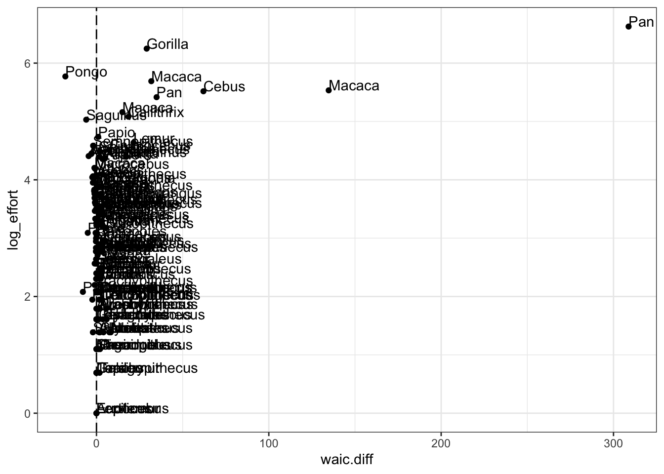
Species on the right of the vertical line fit better for model m3_2, the model with research effort. These are mostly species that are studied a lot, like chimpanzees (Pan) and macaques (Macaca). The genus Pan especially has been a focus on social learning research, and its counts are inflated by this. This is a good example of how the nature of measurement influences inference. There are likely a lot of false zeros in these data, species that are not studied often enough to get a good idea of their learning tendencies. Meanwhile every time a chimpanzee sneezes, someone writes a social learning paper.
3.3
3. Third, draw a DAG to represent how you think the variables social_learning, brain, and research_effort interact. Justify the DAG with the measured associations in the two models above (and any other models you used).
The implied DAG is:
hw6.3dag <- dagitty("dag{
                  S <- E
                  S<- B
                  E <- B
                  }")
plot(hw6.3dag)
## Plot coordinates for graph not supplied! Generating coordinates, see ?coordinates for how to set your own.
B is brain size, E is research effort, and S is social learning. Research effort doesn’t actually influence social learning, but it does influence the value of the variable. The model results above are consistent with this DAG in the sense that including E reduced the association with B, which we would expect when we close the indirect path through E. If researchers choose to look for social learning in species with large brains, this leads to an exaggerated estimate of the association between brains and social learning