Statistical Rethinking 2nd edition Homework 4 in INLA
library(tidyverse)
library(rethinking)
library(dagitty)
library(INLA)
library(knitr)
1. Polynesian islands: compute the entropy of each island’s birb distribution, compute the K-L Divergence of each island from the others, treat- ing each island as if it were a statistical model of the other islands
Consider three fictional Polynesian islands. On each there is a Royal Ornithologist charged by the king with surveying the bird population. They have each found the following proportions of 5 important birb species:
IB1 <- c( 0.2 , 0.2 , 0.2 , 0.2 , 0.2 )
IB2<- c( 0.8 , 0.1 , 0.05 , 0.025 , 0.025 )
IB3 <- c( 0.05 , 0.15 , 0.7 , 0.05 , 0.05 )

df <- data.frame(IB1, IB2, IB3)

rownames(df) <- c("A", "B", "C", "D", "E")

kable(df)| IB1 | IB2 | IB3 | |
|---|---|---|---|
| A | 0.2 | 0.800 | 0.05 |
| B | 0.2 | 0.100 | 0.15 |
| C | 0.2 | 0.050 | 0.70 |
| D | 0.2 | 0.025 | 0.05 |
| E | 0.2 | 0.025 | 0.05 |
Notice that each column sums to 1, all the birbs. This problem has two parts. It is not computationally complicated. But it is conceptually tricky.
First, compute the entropy of each island’s birb distribution. Interpret these entropy values.
Second, use each island’s birb distribution to predict the other two. This means to compute the K-L Divergence of each island from the others, treat- ing each island as if it were a statistical model of the other islands. You should end up with 6 different K-L Divergence values. Which island predicts the others best? Why?
To compute the entropies,we just need a function to compute the entropy.Information entropy, as defined in lecture and the book, is simply: \(H(p) = - \sum_{i}p_i log(p_i)\)
where p is a vector of probabilities summing to 1. In R code this would look like:
H <- function(p) -sum(p*log(p))

IB <- list()
IB[[1]] <- c( 0.2 , 0.2 , 0.2 , 0.2 , 0.2 )
IB[[2]] <- c( 0.8 , 0.1 , 0.05 , 0.025 , 0.025 )
IB[[3]] <- c( 0.05 , 0.15 , 0.7 , 0.05 , 0.05 )
sapply( IB , H )
## [1] 1.6094379 0.7430039 0.9836003The first island has the largest entropy, followed by the third, and then the second in last place. Why is this? Entropy is a measure of the evenness of a distribution. The first islands has the most even distribution of birbs. This means you wouldn’t be very surprised by any particular birb. The second island, in contrast, has a very uneven distribution of birbs. If you saw any birb other than the first species, it would be surprising.
Divergence: The additional uncertainty induced by using probabilities from one distribution to describe another distribution.This is often known as Kullback-Leibler divergence or simply K-L divergence. In plainer language, the divergence is the average difference in log probability between the target (p) and model (q). This divergence is just the difference between two entropies: The entropy of the target distribution p and the cross entropy arising from using q to predict p. When p = q, we know the actual probabilities of the events and the K-L distance = 0. What divergence can do for us now is help us contrast different approximations to p. As an approximating function q becomes more accurate, DKL(p, q) will shrink. So if we have a pair of candidate distributions, then the candidate that minimizes the divergence will be closest to the target. Since predictive models specify probabilities of events (observations), we can use divergence to compare the accuracy of models.
Now we need K-L distance, so let’s write a function for it:
DKL <- function(p,q) sum( p*(log(p)-log(q)) )This is the distance from q to p, regarding p as true and q as the model. Now to use each island as a model of the others, we need to consider the different ordered pairings. I’ll just make a matrix and loop over rows and columns:
Dm <- matrix( NA , nrow=3 , ncol=3 )

for ( i in 1:3 ) for ( j in 1:3 ) Dm[i,j] <- DKL( IB[[j]] , IB[[i]])

#test <- DKL( IB[[1]] , IB[[2]])
#0.2*(log(0.2)- log(0.8)) + 0.2*(log(0.2)- log(0.1))+ 0.2*(log(0.2)- log(0.05))+0.2*(log(0.2)- log(0.025))+0.2*(log(0.2)-log(0.025))

round( Dm , 2 )
## [,1] [,2] [,3]
## [1,] 0.00 0.87 0.63
## [2,] 0.97 0.00 1.84
## [3,] 0.64 2.01 0.00The way to read this is each row as a model and each column as a true distribution. So the first island, the first row, has the smaller distances to the other islands. This makes sense, since it has the highest entropy. Why does that give it a shorter distance to the other islands? Because it is less surprised by the other islands, due to its high entropy.
2. marriage,age,and happiness collider bias
Recall the marriage,age,and happiness collider bias example from Chapter 6.
Consider the question of how aging influences happiness. If we have a large survey of people rating how happy they are, is age associated with happiness? If so, is that association causal?
Suppose, just to be provocative, that an individual’s average happiness is a trait that is determined at birth and does not change with age. However, happiness does influence events in one’s life. One of those events is marriage. Happier people are more likely to get married. Another variable that causally influences marriage is age: The more years you are alive, the more likely you are to eventually get married. Putting these three variables together, this is the causal model:
## Plot coordinates for graph not supplied! Generating coordinates, see ?coordinates for how to set your own.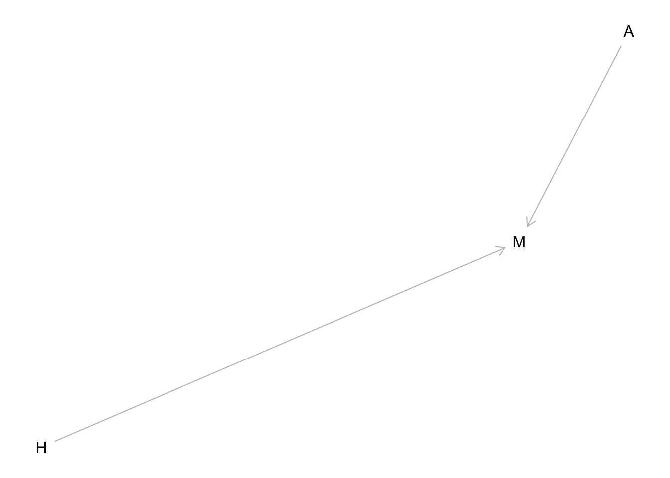
Happiness (H) and age (A) both cause marriage (M). Marriage is therefore a collider. Even though there is no causal association between happiness and age, if we condition on marriage— which means here, if we include it as a predictor in a regression—then it will induce a statistical association between age and happiness. And this can mislead us to think that happiness changes with age, when in fact it is constant.
Run models m6.9 and m6.10 again. Compare these two models using WAIC (or LOO, they will produce identical results). Which model is expected to make better predictions? Which model provides the correct causal inference about the influence of age on happiness? Can you explain why the answers to these two questions disagree?
So let’s consider a multiple regression model aimed at inferring the influence of age on happiness, while controlling for marriage status. This is just a plain multiple regression, like the others in this and the previous chapter.
The linear model is this: \(\mu_i= \alpha mid[i] + \beta AA_i\) where mid[i] is an index for the marriage status of individual i, with 1 meaning single and 2 meaning married. It’s easier to make priors, when we use multiple intercepts, one for each category, than when we use indicator variables.
Now we should do our duty and think about the priors.
Let’s consider the slope \(\beta A\) first, because how we scale the predictor A will determine the meaning of the intercept. We’ll focus only on the adult sample, those 18 or over. Imagine a very strong relationship between age and happiness, such that happiness is at its maximum at age 18 and its minimum at age 65. It’ll be easier if we rescale age so that the range from 18 to 65 is one unit. Now this new variable A ranges from 0 to 1, where 0 is age 18 and 1 is age 65.
Happiness is on an arbitrary scale, in these data, from −2 to +2. So our imaginary strongest relationship, taking happiness from maximum to minimum, has a slope with rise over run of (2 − (−2))/1 = 4. Remember that 95% of the mass of a normal distribution is contained within 2 standard deviations. So if we set the standard deviation of the prior to half of 4, we are saying that we expect 95% of plausible slopes to be less than maximally strong. That isn’t a very strong prior, but again, it at least helps bound inference to realistic ranges.
Now for the intercepts. Each α is the value of \(\mu_i\) when Ai = 0. In this case, that means at age 18. So we need to allow \(\alpha\) to cover the full range of happiness scores. Normal(0, 1) will put 95% of the mass in the −2 to +2 interval.
We need to construct the marriage status index variable, as well.
Finally, let’s approximate the posterior.
d <- sim_happiness( seed=1977 , N_years=1000 )
d2 <- d[ d$age>17 , ] # only adults
d2$A <- ( d2$age - 18 ) / ( 65 - 18 )
d2$mid <- d2$married + 1
Model m6.9 contains both marriage status and age. Model m6.10 contains only age. Model m6.9 produces a confounded inference about the relationship between age and happiness, due to opening a collider path.
2.1 marriage status and age
2.1 rethinking
#contains both marriage status and age

m6.9 <- quap(
    alist(
        happiness ~ dnorm( mu , sigma ),
        mu <- a[mid] + bA*A,
        a[mid] ~ dnorm( 0 , 1 ),
        bA ~ dnorm( 0 , 2 ),
        sigma ~ dexp(1)
    ) , data=d2 )
precis(m6.9,depth=2)
## mean sd 5.5% 94.5%
## a[1] -0.2350877 0.06348986 -0.3365568 -0.1336186
## a[2] 1.2585517 0.08495989 1.1227694 1.3943340
## bA -0.7490274 0.11320112 -0.9299447 -0.5681102
## sigma 0.9897080 0.02255800 0.9536559 1.02576002.1 INLA
In order to code a separate intercept for being married/not, we need to reformat the data so that there are separate variables for each intercept, with 1s for a given value of the variable we are basing the intercept on ( in this case marriage) and NAs for all other values.
d3 <- d2 %>%
  mutate(i_notmarried= na_if(if_else(married==0, 1, 0), 0),
         i_married= na_if(married, 0))

m6.9.inla.prior <- inla(happiness~ -1 +i_notmarried+i_married + A , data= d3,
                        control.fixed = list(
        mean= 0,
        prec= list(i_notmarried=2, i_married= 1, A=2)),
        control.compute = list(dic=TRUE, waic= TRUE)
)

summary(m6.9.inla.prior )
##
## Call:
## c("inla(formula = happiness ~ -1 + i_notmarried + i_married + A, ", "
## data = d3, control.compute = list(dic = TRUE, waic = TRUE), ", "
## control.fixed = list(mean = 0, prec = list(i_notmarried = 2, ", "
## i_married = 1, A = 2)))")
## Time used:
## Pre = 1.24, Running = 0.454, Post = 0.222, Total = 1.91
## Fixed effects:
## mean sd 0.025quant 0.5quant 0.975quant mode kld
## i_notmarried -0.240 0.063 -0.364 -0.240 -0.116 -0.240 0
## i_married 1.251 0.084 1.085 1.251 1.416 1.251 0
## A -0.736 0.112 -0.956 -0.736 -0.516 -0.736 0
##
## Model hyperparameters:
## mean sd 0.025quant 0.5quant
## Precision for the Gaussian observations 1.02 0.046 0.93 1.02
## 0.975quant mode
## Precision for the Gaussian observations 1.11 1.02
##
## Expected number of effective parameters(stdev): 2.97(0.002)
## Number of equivalent replicates : 323.69
##
## Deviance Information Criterion (DIC) ...............: 2714.19
## Deviance Information Criterion (DIC, saturated) ....: 967.05
## Effective number of parameters .....................: 4.00
##
## Watanabe-Akaike information criterion (WAIC) ...: 2713.83
## Effective number of parameters .................: 3.62
##
## Marginal log-Likelihood: -1374.21
## Posterior marginals for the linear predictor and
## the fitted values are computed2.2 only age
2.2 rethinking
#this model to a model that omits marriage status.
m6.10 <- quap(
    alist(
        happiness ~ dnorm( mu , sigma ),
        mu <- a + bA*A,
        a ~ dnorm( 0 , 1 ),
        bA ~ dnorm( 0 , 2 ),
        sigma ~ dexp(1)
    ) , data=d2 )
precis(m6.10)
## mean sd 5.5% 94.5%
## a -1.469528e-06 0.07675016 -0.1226630 0.1226601
## bA 2.378318e-06 0.13225977 -0.2113743 0.2113790
## sigma 1.213188e+00 0.02766081 1.1689804 1.25739502.2 INLA
m6.10.inla.prior <- inla(happiness~ A , data= d3,
                        control.fixed = list(
        mean= 0,
        prec= 1/(2^2),
        mean.intercept= 0,
        prec.intercept= 1),
        control.compute = list(dic=TRUE, waic= TRUE)
)

summary(m6.10.inla.prior )
##
## Call:
## c("inla(formula = happiness ~ A, data = d3, control.compute = list(dic
## = TRUE, ", " waic = TRUE), control.fixed = list(mean = 0, prec =
## 1/(2^2), ", " mean.intercept = 0, prec.intercept = 1))")
## Time used:
## Pre = 1.18, Running = 0.466, Post = 0.205, Total = 1.85
## Fixed effects:
## mean sd 0.025quant 0.5quant 0.975quant mode kld
## (Intercept) 0 0.077 -0.151 0 0.151 0 0
## A 0 0.132 -0.260 0 0.260 0 0
##
## Model hyperparameters:
## mean sd 0.025quant 0.5quant
## Precision for the Gaussian observations 0.679 0.031 0.62 0.678
## 0.975quant mode
## Precision for the Gaussian observations 0.74 0.677
##
## Expected number of effective parameters(stdev): 1.99(0.001)
## Number of equivalent replicates : 481.52
##
## Deviance Information Criterion (DIC) ...............: 3102.67
## Deviance Information Criterion (DIC, saturated) ....: 966.07
## Effective number of parameters .....................: 3.03
##
## Watanabe-Akaike information criterion (WAIC) ...: 3102.05
## Effective number of parameters .................: 2.41
##
## Marginal log-Likelihood: -1566.72
## Posterior marginals for the linear predictor and
## the fitted values are computedTo compare these models using WAIC:
compare rethinking
#rethinking
 compare( m6.9 , m6.10 )
## WAIC SE dWAIC dSE pWAIC weight
## m6.9 2713.964 37.55324 0.0000 NA 3.732484 1.000000e+00
## m6.10 3101.906 27.74820 387.9425 35.41158 2.337316 5.745894e-85compare INLA
m6.9.inla.prior$waic$waic## [1] 2713.829m6.10.inla.prior$waic$waic## [1] 3102.055The model that produces the invalid inference, m6.9, is expected to predict much better. And it would. This is because the collider path does convey actual association. We simply end up mistaken about the causal inference. We should not use WAIC (or LOO) to choose among models, unless we have some clear sense of the causal model. These criteria will happily favor confounded models.
3. data(fexes) Use WAIC or LOO based model comparison on five different models
Reconsider the urban fox analysis from last week’s homework. Use WAIC or LOO based model comparison on five different models, each using weight as the outcome, and containing these sets of predictor variables: (1) avgfood + groupsize + area (2) avgfood + groupsize (3) groupsize + area (4) avgfood (5) area
Can you explain the relative differences in WAIC scores, using the fox DAG from last week’s homework? Be sure to pay attention to the standard error of the score differences (dSE).
## Plot coordinates for graph not supplied! Generating coordinates, see ?coordinates for how to set your own.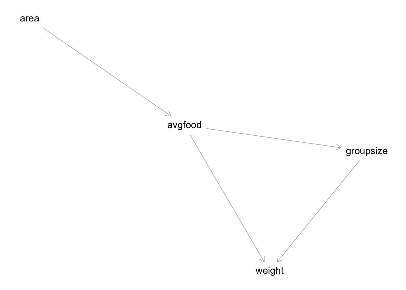
library(rethinking)
data(foxes)
d <- foxes
d$W <- standardize(d$weight)
d$A <- standardize(d$area)
d$F <- standardize(d$avgfood)
d$G <- standardize(d$groupsize)
3. rethinking
m1 <- quap(
    alist(
        W ~ dnorm( mu , sigma ),
        mu <- a + bF*F + bG*G + bA*A,
        a ~ dnorm(0,0.2),
        c(bF,bG,bA) ~ dnorm(0,0.5),
        sigma ~ dexp(1)
    ), data=d )
m2 <- quap(
    alist(
        W ~ dnorm( mu , sigma ),
        mu <- a + bF*F + bG*G,
        a ~ dnorm(0,0.2),
        c(bF,bG) ~ dnorm(0,0.5),
        sigma ~ dexp(1)
    ), data=d )
m3 <- quap(
    alist(
        W ~ dnorm( mu , sigma ),
        mu <- a + bG*G + bA*A,
        a ~ dnorm(0,0.2),
        c(bG,bA) ~ dnorm(0,0.5),
        sigma ~ dexp(1)
    ), data=d )
m4 <- quap(
    alist(
        W ~ dnorm( mu , sigma ),
        mu <- a + bF*F,
        a ~ dnorm(0,0.2),
        bF ~ dnorm(0,0.5),
        sigma ~ dexp(1)
    ), data=d )
m5 <- quap(
    alist(
        W ~ dnorm( mu , sigma ),
        mu <- a + bA*A,
        a ~ dnorm(0,0.2),
        bA ~ dnorm(0,0.5),
        sigma ~ dexp(1)
), data=d )


 compare( m1 , m2 , m3 , m4 , m5 )
## WAIC SE dWAIC dSE pWAIC weight
## m1 322.8570 16.27702 0.000000 NA 4.643026 0.464863619
## m3 323.8852 15.67222 1.028262 2.911577 3.711944 0.277997758
## m2 324.0754 16.12771 1.218433 3.584892 3.818873 0.252782029
## m4 333.4369 13.78791 10.579891 7.194478 2.423844 0.002343859
## m5 333.7415 13.79359 10.884499 7.243278 2.659040 0.0020127353. INLA
m1.i <- inla(W~F+G+A, data= d, control.fixed = list(
        mean= list(0),
        prec= list(F=1/(0.5^2), G=1/(0.5^2), A= 1/(0.5^2)),
        mean.intercept= 0,
        prec.intercept= 1/(0.2^2)
),
control.compute = list(waic= TRUE))
#summary(m1.i)

m2.i <- inla(W~F+G, data= d, control.fixed = list(
        mean= list(0),
        prec= list(F=1/(0.5^2), G=1/(0.5^2)),
        mean.intercept= 0,
        prec.intercept= 1/(0.2^2)
),
control.compute = list(waic= TRUE))
#summary(m2.i)

m3.i <- inla(W~A+G, data= d, control.fixed = list(
        mean= list(0),
        prec= list(A=1/(0.5^2), G=1/(0.5^2)),
        mean.intercept= 0,
        prec.intercept= 1/(0.2^2)
),
control.compute = list(waic= TRUE))
#summary(m3.i)

m4.i <- inla(W~F, data= d, control.fixed = list(
        mean= 0,
        prec= 1/(0.5^2),
        mean.intercept= 0,
        prec.intercept= 1/(0.2^2)
),
control.compute = list(waic= TRUE))
#summary(m4.i)

m5.i <- inla(W~A, data= d, control.fixed = list(
        mean= 0,
        prec= 1/(0.5^2),
        mean.intercept= 0,
        prec.intercept= 1/(0.2^2)
),
control.compute = list(waic= TRUE))
#summary(m5.i)

m1.i$waic$waic
## [1] 322.9293m2.i$waic$waic## [1] 323.6849m3.i$waic$waic## [1] 323.767m4.i$waic$waic## [1] 333.412m5.i$waic$waic## [1] 333.6651Notice that the top three models are m1, m3, and m2. They have very similar WAIC values. The differences are small and smaller in all cases than the standard error of the difference. WAIC sees these models are tied. This makes sense, given the DAG, because as long as a model has groupsize in it, we can include either avgfood or area or both and get the same inferences. Another way to think of this is that the influence of good, adjusting for group size, is (according to the DAG) the same as the influence of area, adjusting for group size, because the influence of area is routed entirely through food and group size. There are no backdoor paths. What about the other two models, m4 and m5? These models are tied with one another, and both omit group size. Again, the influence of area passes entirely through food. So including only food or only area should produce the same inference—the total causal influence of area (or food) is just about zero. That’s indeed what the posterior distributions suggest:
coeftab(m4,m5)## m4 m5
## a 0 0
## bF -0.02 NA
## sigma 0.99 0.99
## bA NA 0.02
## nobs 116 116