library(tidyverse)
library(rethinking)
library(dagitty)
library(INLA)

All three problems below are based on the same data. The data in data(foxes) are 116 foxes from 30 different urban groups in England. These foxes are like street gangs. Group size varies from 2 to 8 individuals. Each group maintains its own (almost exclusive) urban territory. Some territories are larger than others. The area variable encodes this information. Some territories also have more avgfood than others. We want to model the weight of each fox. For the problems below, assume this DAG:

hw3dag <- dagitty("dag{
                  avgfood <- area
                  weight <- avgfood
                  weight <- groupsize
                  groupsize <- avgfood
                  }")

plot(hw3dag)

## Plot coordinates for graph not supplied! Generating coordinates, see ?coordinates for how to set your own.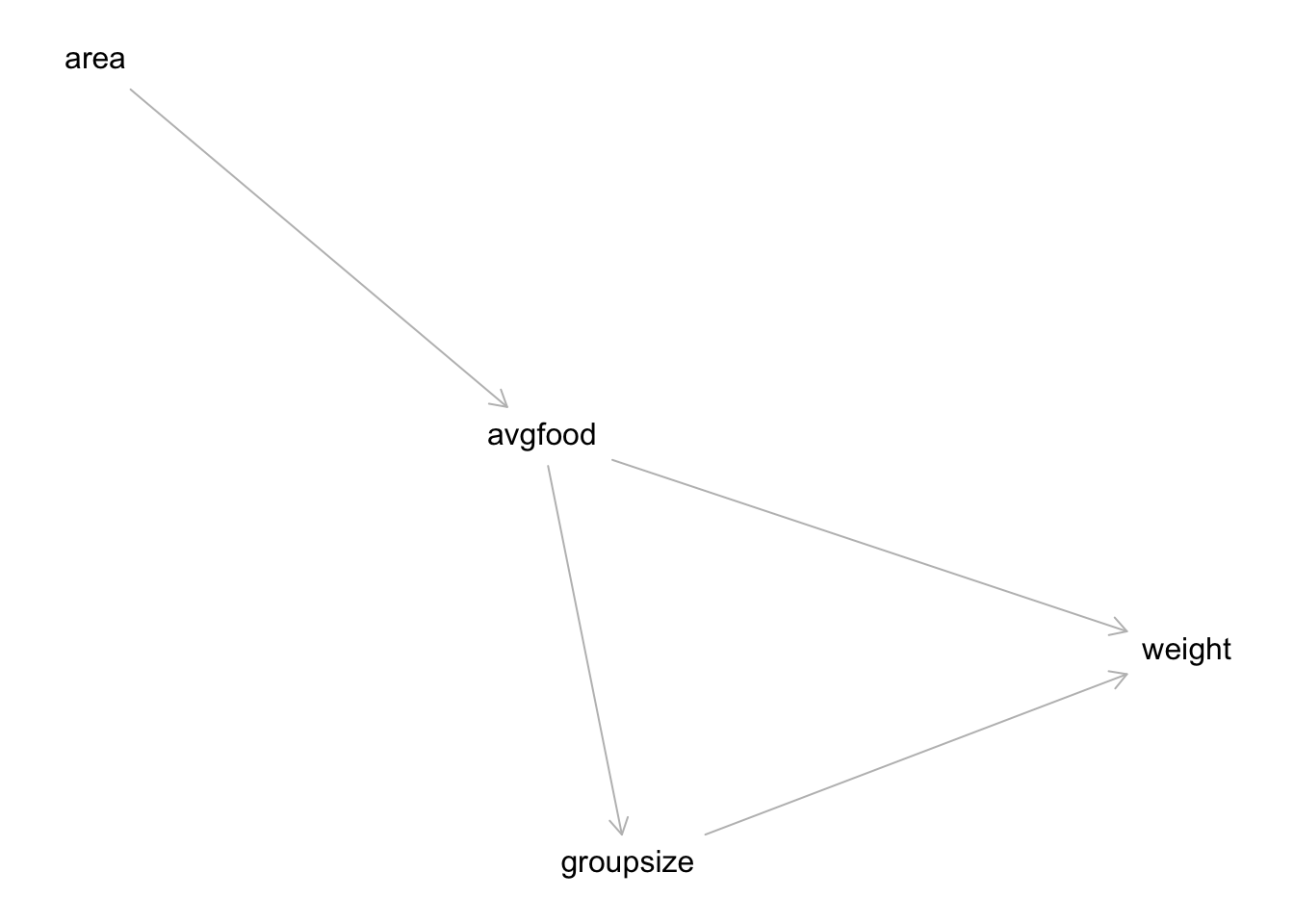

1. data(foxes) infer the total causal influence of area on weight

Use a model to infer the total causal influence of area on weight. Would increasing the area available to each fox make it heavier (healthier)? You might want to standardize the variables. Regardless, use prior predictive simulation to show that your model’s prior predictions stay within the possible outcome range.

1. rethinking

Because there are no back-door paths from area to weight,we only need to include area. No other variables are needed. Territory size seems to have no total causal influence on weight, at least not in this sample.

data(foxes)
f <- foxes

f$A <- scale( f$area )
f$F <- scale( f$avgfood )
f$G <- scale( f$groupsize )
f$W <- scale( f$weight)

m1 <- quap(
    alist(
        W ~ dnorm( mu , sigma ) ,
        mu <- a + bA*A ,
        a ~ dnorm( 0 , 0.2 ) ,
        bA ~ dnorm( 0 , 0.5 ) ,
        sigma ~ dexp( 1 )
) , data=f )

precis(m1)

##                mean         sd       5.5%     94.5%
## a     -2.483642e-05 0.08360740 -0.1336456 0.1335959
## bA     1.886254e-02 0.09089420 -0.1264040 0.1641290
## sigma  9.912479e-01 0.06466352  0.8879031 1.0945927

1. INLA

default priors

By default, the intercept has a Gaussian prior with mean and precision equal to zero. Coefficients of the fixed effects also have a Gaussian prior by default with zero mean and precision equal to
0.001. The prior on the precision of the error term is, by default, a Gamma distribution with parameters 1 and 0.00005 (shape and rate, respectively) ( so this is different from the statistical rethinking book’s prior on the variance which is exp(1))

#using default priors

m1.inla <- inla(W~A, data= f)
summary(m1.inla)

## 
## Call:
##    "inla(formula = W ~ A, data = f)" 
## Time used:
##     Pre = 2.01, Running = 0.133, Post = 0.146, Total = 2.29 
## Fixed effects:
##              mean    sd 0.025quant 0.5quant 0.975quant  mode kld
## (Intercept) 0.000 0.093     -0.183    0.000      0.183 0.000   0
## A           0.019 0.094     -0.165    0.019      0.203 0.019   0
## 
## Model hyperparameters:
##                                         mean    sd 0.025quant 0.5quant
## Precision for the Gaussian observations 1.01 0.132      0.767     1.00
##                                         0.975quant  mode
## Precision for the Gaussian observations       1.28 0.992
## 
## Expected number of effective parameters(stdev): 2.00(0.00)
## Number of equivalent replicates : 57.98 
## 
## Marginal log-Likelihood:  -182.37

The precision is the inverse of the variance. If we want to set the sd to 0.5, we have to set the precision to 1/(0.5^2)

m1.inla.prior <- inla(W~A, data= f, control.fixed = list(
        mean= 0, 
        prec= 1/(0.5^2), # sd = 0.5 --> precision =1/variance --> 1/(sd^2)
        mean.intercept= 0, 
        prec.intercept= 1/(0.2^2)
))

summary(m1.inla.prior)

## 
## Call:
##    c("inla(formula = W ~ A, data = f, control.fixed = list(mean = 0, ", " 
##    prec = 1/(0.5^2), mean.intercept = 0, prec.intercept = 1/(0.2^2)))" ) 
## Time used:
##     Pre = 1.17, Running = 0.133, Post = 0.136, Total = 1.44 
## Fixed effects:
##              mean    sd 0.025quant 0.5quant 0.975quant  mode kld
## (Intercept) 0.000 0.084     -0.166    0.000      0.166 0.000   0
## A           0.019 0.092     -0.162    0.019      0.199 0.019   0
## 
## Model hyperparameters:
##                                         mean    sd 0.025quant 0.5quant
## Precision for the Gaussian observations 1.01 0.132      0.769     1.00
##                                         0.975quant  mode
## Precision for the Gaussian observations       1.29 0.993
## 
## Expected number of effective parameters(stdev): 1.79(0.025)
## Number of equivalent replicates : 64.84 
## 
## Marginal log-Likelihood:  -177.65

2. data(foxes) infer the causal impact of adding food to a territory

Now infer the causal impact of adding food to a territory. Would this make foxes heavier? Which covariates do you need to adjust for to estimate the total causal influence of food?

2.rethinking

To infer the causal influence of avg food on weight,we need to close any back-door paths. There are no back-door paths in the DAG. So again, just use a model with a single predictor. If you include groupsize, to block the indirect path, then you won’t get the total causal influence of food. You’ll just get the direct influence. But I asked for the effect of adding food, and that would mean through all forward paths.

Again nothing. Adding food does not change weight. This shouldn’t surprise you, if the DAG is correct, because area is upstream of avgfood.

# food on weight
m2 <- quap(
    alist(
        W ~ dnorm( mu , sigma ) ,
        mu <- a + bF*F,
        a ~ dnorm( 0 , 0.2 ) ,
        bF ~ dnorm( 0 , 0.5 ) ,
        sigma ~ dexp( 1 )
) , data=f )

precis(m2)

##                mean         sd       5.5%     94.5%
## a      1.686958e-07 0.08360013 -0.1336090 0.1336093
## bF    -2.421092e-02 0.09088496 -0.1694626 0.1210408
## sigma  9.911433e-01 0.06465848  0.8878066 1.0944801

2.INLA

INLA default priors

#using default priors

m2.inla <- inla(W~F, data= f)
summary(m2.inla)

## 
## Call:
##    "inla(formula = W ~ F, data = f)" 
## Time used:
##     Pre = 1.19, Running = 0.132, Post = 0.139, Total = 1.46 
## Fixed effects:
##               mean    sd 0.025quant 0.5quant 0.975quant   mode kld
## (Intercept)  0.000 0.093     -0.183    0.000      0.183  0.000   0
## F           -0.025 0.094     -0.209   -0.025      0.159 -0.025   0
## 
## Model hyperparameters:
##                                         mean    sd 0.025quant 0.5quant
## Precision for the Gaussian observations 1.01 0.132      0.767     1.00
##                                         0.975quant  mode
## Precision for the Gaussian observations       1.28 0.992
## 
## Expected number of effective parameters(stdev): 2.00(0.00)
## Number of equivalent replicates : 57.98 
## 
## Marginal log-Likelihood:  -182.36

INLA custom priors

#using custom priors

m2.prec.prior <-  
    
m2.inla.prior <- inla(W~F, data= f, control.fixed = list(
        mean= 0, 
        prec= 1/(0.5^2), 
        mean.intercept= 0, 
        prec.intercept= 1/(0.2^2)
))
summary(m2.inla.prior)

## 
## Call:
##    c("inla(formula = W ~ F, data = f, control.fixed = list(mean = 0, ", " 
##    prec = 1/(0.5^2), mean.intercept = 0, prec.intercept = 1/(0.2^2)))" ) 
## Time used:
##     Pre = 1.22, Running = 0.131, Post = 0.149, Total = 1.5 
## Fixed effects:
##               mean    sd 0.025quant 0.5quant 0.975quant   mode kld
## (Intercept)  0.000 0.084     -0.166    0.000      0.166  0.000   0
## F           -0.024 0.092     -0.205   -0.024      0.156 -0.024   0
## 
## Model hyperparameters:
##                                         mean    sd 0.025quant 0.5quant
## Precision for the Gaussian observations 1.01 0.132      0.769     1.00
##                                         0.975quant  mode
## Precision for the Gaussian observations       1.29 0.994
## 
## Expected number of effective parameters(stdev): 1.79(0.025)
## Number of equivalent replicates : 64.84 
## 
## Marginal log-Likelihood:  -177.64

3. data(foxes) infer the causal impact of groupsize

Now infer the causal impact of groupsize. Which covariates do you need to adjust for? Looking at the posterior distribution of the resulting model, what do you think explains these data? That is, can you explain the estimates for all three problems? How do they go together?

3. rethinking

The variable groupsize does have a back-door path, passing through avgfood. So to infer the causal influence of groupsize, we need to close that path. This implies a model with both groupsize and avgfood as predictors.

It looks like group size is negatively associated with weight, controlling for food. Similarly, food is positively associated with weight, controlling for group size. So the causal influence of group size is to reduce weight—less food for each fox. And the direct causal influence of food is positive, of course. But the total causal influence of food is still nothing, since it causes larger groups. This is a masking effect, like in the milk energy example. But the causal explanation here is that more foxes move into a territory until the food available to each is no better than the food in a neighboring territory. Every territory ends up equally good/bad on average. This is known in be- havioral ecology as an ideal free distribution.

# groupsize on weight
#need to include avgfood
m3 <- quap(
    alist(
        W ~ dnorm( mu , sigma ) ,
        mu <- a + bF*F + bG*G,
        a ~ dnorm( 0 , 0.2 ) ,
        bF ~ dnorm( 0 , 0.5 ) ,
        bG ~ dnorm( 0 , 0.5 ) ,
        sigma ~ dexp( 1 )
) , data=f )

precis(m3)

##                mean         sd       5.5%      94.5%
## a     -9.170948e-05 0.08013639 -0.1281651  0.1279817
## bF     4.772661e-01 0.17911961  0.1909984  0.7635339
## bG    -5.735298e-01 0.17913821 -0.8598273 -0.2872324
## sigma  9.420204e-01 0.06174870  0.8433340  1.0407067

3. INLA