Statistical Rethinking 2nd edition Homework 9 in INLA
library(tidyverse)
library(rethinking)
library(dagitty)
library(INLA)
library(knitr)
library(stringr)
1. data(bangladesh) model with both varying intercepts by district_id and varying slopes of urban (as a 0/1 indicator variable) by district_id and correlation between the intercepts and slopes
Revisit the Bangladesh fertility data, data(bangladesh).Fit a model with both varying intercepts by district_id and varying slopes of urban (as a 0/1 indicator variable) by district_id. You are still predicting use.contraception. Inspect the correlation between the intercepts and slopes. Can you interpret this correlation, in terms of what it tells you about the pattern of contraceptive use in the sample? It might help to plot the varying effect estimates for both the intercepts and slopes, by district. Then you can visualize the correlation and maybe more easily think through what it means to have a particular correlation. Plotting predicted proportion of women using contraception, in each district, with urban women on one axis and rural on the other, might also help.
1.1 model varying slopes of urban
\(C_{did} \sim Bernoulli(p_{did})\)
\(logit(p_{did}) = \alpha_{did} + \beta_{did}*urban_{did}\)
\(\begin{pmatrix}a_{did}\\b_{did}\end{pmatrix}= MVNormal \begin{pmatrix}\left[\begin{array}{ccc}\bar{a}\\\bar{b}\end{array}\right] , & Sigma ,& Rho\end{pmatrix}\)
1.1 rethinking
library(rethinking)
data(bangladesh)
d <- bangladesh

dat_list <- list(
C = d$use.contraception,
did = as.integer( as.factor(d$district) ),
urban = d$urban
)

m1.1 <- ulam(
  alist(
C ~ bernoulli( p ),
logit(p) <- a[did] + b[did]*urban,
c(a,b)[did] ~ multi_normal( c(abar,bbar) , Rho , Sigma ),
abar ~ normal(0,1),
bbar ~ normal(0,0.5),
Rho ~ lkj_corr(2),
Sigma ~ exponential(1)
) , data=dat_list , chains=4 , cores=4 )
## Warning: The largest R-hat is NA, indicating chains have not mixed.
## Running the chains for more iterations may help. See
## http://mc-stan.org/misc/warnings.html#r-hat## Warning: Bulk Effective Samples Size (ESS) is too low, indicating posterior means and medians may be unreliable.
## Running the chains for more iterations may help. See
## http://mc-stan.org/misc/warnings.html#bulk-essprecis(m1.1)## mean sd 5.5% 94.5% n_eff Rhat4
## abar -0.6865358 0.1017140 -0.8472127 -0.5281305 1680.789 0.9996217
## bbar 0.6427001 0.1581673 0.3919394 0.8948358 1159.847 0.9997477This is a conventional varying slopes model, with a centered parameterization. No surprises. If you peek at the posterior distributions for the average effects, you’ll see that the average slope is positive. This implies that urban areas use contraception more. Not surprising.
Now consider the distribution of varying effects:
precis( m1.1 , depth=3 , pars=c("Rho","Sigma") )## mean sd 5.5% 94.5% n_eff Rhat4
## Rho[1,1] 1.0000000 0.000000e+00 1.0000000 1.0000000 NaN NaN
## Rho[1,2] -0.6546999 1.671207e-01 -0.8699901 -0.3556045 247.3203 1.023925
## Rho[2,1] -0.6546999 1.671207e-01 -0.8699901 -0.3556045 247.3203 1.023925
## Rho[2,2] 1.0000000 5.918041e-17 1.0000000 1.0000000 1232.7053 0.997998
## Sigma[1] 0.5748587 1.001156e-01 0.4299495 0.7461187 639.2464 1.010080
## Sigma[2] 0.7737014 1.920344e-01 0.4755791 1.0783823 248.7727 1.027379The correlation between the intercepts and slopes is quite negative.
Let’s plot the individual effects to appreciate this.
post <- extract.samples(m1.1)

a <- apply( post$a , 2 , mean )
b <- apply( post$b , 2 , mean )
plot( a, b , xlab="a (intercept)" , ylab="b (urban slope)" )
abline( h=0 , lty=2 )
abline( v=0 , lty=2 )
library(ellipse)
R <- apply( post$Rho , 2:3 , mean )
s <- apply( post$Sigma , 2 , mean )
S <- diag(s) %*% R %*% diag(s)
ll <- c( 0.5 , 0.67 , 0.89 , 0.97 )
for ( l in ll ) {
el <- ellipse( S , centre=c( mean(post$abar) , mean(post$bbar) ) , level=l )
lines( el , col="black" , lwd=0.5 ) }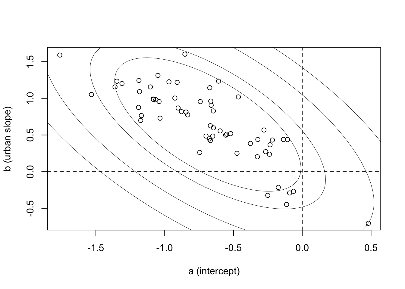
There’s the negative correlation — districts with higher use outside urban areas (a values) have smaller slopes. Since the slope is the difference between urban and non-urban areas, you can see this as saying that districts with high use in rural areas have urban areas that aren’t as different.
On the outcome scale, what this ends up meaning is that urban places are much the same in all districts, but rural areas vary a lot. Plotting now in the outcome scale:
u0 <- inv_logit( a )
u1 <- inv_logit( a + b )
plot( u0 , u1 , xlim=c(0,1) , ylim=c(0,1) , xlab="urban = 0" , ylab="urban = 1" )
abline( h=0.5 , lty=2 )
abline( v=0.5 , lty=2 )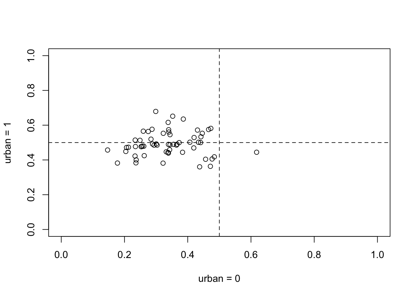
This plot is on the probability scale. The horizontal axis is probability of contraceptive use in rural area of a district. The vertical is the probability in urban area of same district. The urban areas all straddle 0.5. Most the of the rural areas are below 0.5. The negative correlation between the intercepts and slopes is necessary to encode this pattern.
1.1. inla
library(INLA)
library(brinla)

d1.i <- d %>%
  #make a new variable of district that is continuous
  mutate(C = use.contraception,
         did = as.integer( as.factor(d$district)),
         a.did= did,
         b.did= did + max(did)
  )

n.district= max(d1.i$did) ## = 60


m1.1.i <- inla(C ~ 1 + urban + f(a.did, model="iid2d", n= 2*n.district) + f(b.did, urban, copy= "a.did"), data= d1.i, family = "binomial",
              Ntrials = 1,
              control.fixed = list(
        mean= 0,
        prec= 1/(0.5^2),
        mean.intercept= 0,
        prec.intercept= 1),
              control.family = list(control.link=list(model="logit")),
              control.predictor=list(link=1, compute=T),
              control.compute=list(config=T, dic=TRUE, waic= TRUE))
summary(m1.1.i)
##
## Call:
## c("inla(formula = C ~ 1 + urban + f(a.did, model = \"iid2d\", n = 2 *
## ", " n.district) + f(b.did, urban, copy = \"a.did\"), family =
## \"binomial\", ", " data = d1.i, Ntrials = 1, control.compute =
## list(config = T, ", " dic = TRUE, waic = TRUE), control.predictor =
## list(link = 1, ", " compute = T), control.family = list(control.link =
## list(model = \"logit\")), ", " control.fixed = list(mean = 0, prec =
## 1/(0.5^2), mean.intercept = 0, ", " prec.intercept = 1))")
## Time used:
## Pre = 1.81, Running = 2.83, Post = 0.396, Total = 5.04
## Fixed effects:
## mean sd 0.025quant 0.5quant 0.975quant mode kld
## (Intercept) -0.686 0.099 -0.884 -0.686 -0.492 -0.685 0
## urban 0.639 0.157 0.331 0.639 0.950 0.638 0
##
## Random effects:
## Name Model
## a.did IID2D model
## b.did Copy
##
## Model hyperparameters:
## mean sd 0.025quant 0.5quant 0.975quant
## Precision for a.did (component 1) 3.115 1.029 1.582 2.955 5.572
## Precision for a.did (component 2) 1.921 0.936 0.709 1.723 4.278
## Rho1:2 for a.did -0.664 0.146 -0.874 -0.689 -0.312
## mode
## Precision for a.did (component 1) 2.66
## Precision for a.did (component 2) 1.39
## Rho1:2 for a.did -0.74
##
## Expected number of effective parameters(stdev): 51.59(5.30)
## Number of equivalent replicates : 37.49
##
## Deviance Information Criterion (DIC) ...............: 2467.53
## Deviance Information Criterion (DIC, saturated) ....: 2467.53
## Effective number of parameters .....................: 52.66
##
## Watanabe-Akaike information criterion (WAIC) ...: 2467.09
## Effective number of parameters .................: 50.50
##
## Marginal log-Likelihood: -1252.49
## Posterior marginals for the linear predictor and
## the fitted values are computedbri.hyperpar.summary(m1.1.i)## mean sd q0.025 q0.5
## SD for a.did (component 1) 0.5887788 0.09423246 0.4243071 0.5816066
## SD for a.did (component 2) 0.7805681 0.17929237 0.4843403 0.7614524
## Rho1:2 for a.did -0.6636992 0.14555091 -0.8738944 -0.6895578
## q0.975 mode
## SD for a.did (component 1) 0.7934828 0.5683934
## SD for a.did (component 2) 1.1851196 0.7251542
## Rho1:2 for a.did -0.3135566 -0.7405877bri.hyperpar.plot(m1.1.i)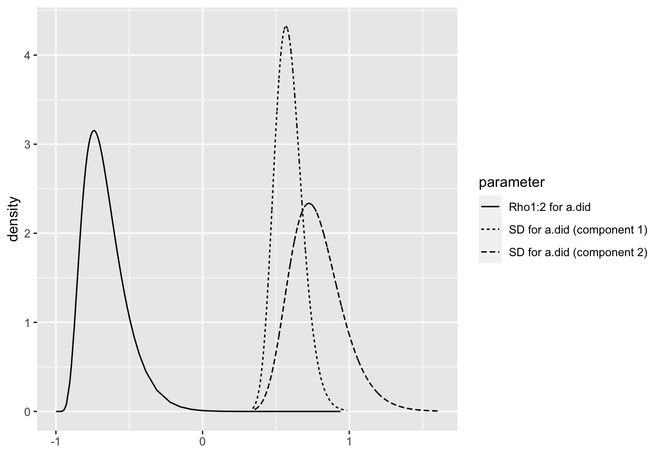
#m1.1.i$summary.random has 2 elements: a.did and b.did but they are identical.

#extract the means of the random effects with m1.1.i$summary.random[[1]][["mean"]]
m1.1.i.mean <- bind_cols(did= 1:length(m1.1.i$summary.random[[1]][["mean"]]), mean= m1.1.i$summary.random[[1]][["mean"]]) %>%
  #assign first 60 rows to a.did and 61:120 to b.did in new variable "param"
  mutate(param= if_else(did <= n.district, "a.did", "b.did"),
         #new variable "district" assigns the district index 1:60 to both a.did and b.did estimates.
         district= rep(1:60,2)) %>%
  #split dataframe by param into a list of 2: a.did and b.did
  group_split(param) %>%
  #join the a.did and b.did elements of the list into a dataframe by "district"
  reduce(left_join, by= "district") %>%
  select(c( "district", "mean.x", "mean.y")) %>%
  rename("a.did"= "mean.x", "b.did"= "mean.y") %>%
  mutate(intercept= a.did + m1.1.i$summary.fixed[[1]][[1]],
         slope= b.did + m1.1.i$summary.fixed[[1]][[2]])


m1.1.i.mean.plot <-  ggplot()+
  geom_point(data= m1.1.i.mean, aes(x=intercept, y= slope))+
  geom_hline(yintercept=0, linetype='longdash') +
  geom_vline(xintercept = 0)+
  labs(x= "a (intercept)", y = "b (urban slope)")+
  theme_bw()

m1.1.i.mean.plot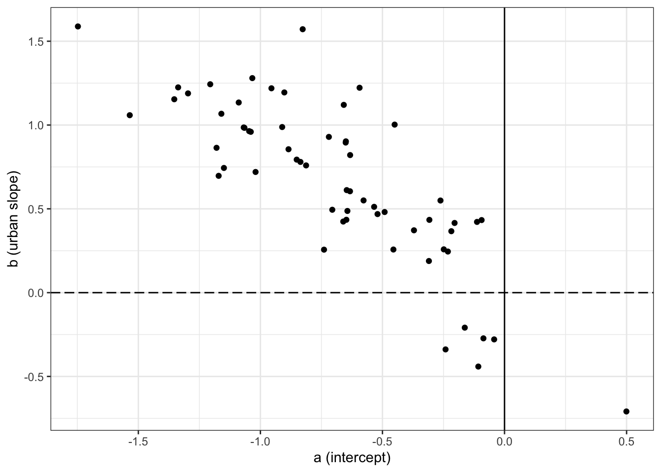
inverse_logit <- function (x){
    p <- 1/(1 + exp(-x))
    p <- ifelse(x == Inf, 1, p)
    p }


m1.1.i.outcome <- m1.1.i.mean %>%
  mutate(u0.i = inverse_logit(a.did + m1.1.i$summary.fixed[[1]][[1]]),
         u1.i= inverse_logit(a.did + m1.1.i$summary.fixed[[1]][[1]] +
                               b.did + m1.1.i$summary.fixed[[1]][[2]])
         )


m1.1.i.outcome.plot <-  ggplot()+
  geom_point(data= m1.1.i.outcome, aes(x=u0.i, y= u1.i))+
  geom_hline(yintercept=0.5, linetype='longdash') +
  geom_vline(xintercept = 0.5)+
  labs(x= "urban = 0", y = "urban = 1")+
  xlim(0,1) +
  ylim(0,1)+
  theme_bw()

m1.1.i.outcome.plot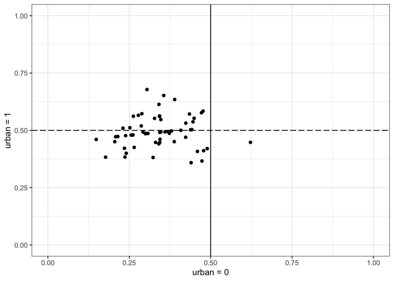
Difference between the rethinking and INLA model parametrization
The rethinking random effects are parameterized like N[ (a, b); Sigma ], while the INLA random effects are parameterized like (a, b) + N[ (0, 0); Sigma ]. From INLA’s perspective, (a, b) are fixed effects that define the center of the random effect. The INLA plot is centered at (0,0), while in this case, the rethinking plot is centered at (-0.68, 0.65). That’s why, when we want to replicate the rethinking model in INLA, we have to add the the fixed effects, which are the center of the distribution, to the random effects, which are deviations from that center.
Example:
m1.1.i$summary.fixed[[1]][[1]] is the fixed effect of the intercept a.did is the deviation from the intercept by district
a.did + m1.1.i$summary.fixed[[1]][[1]] in INLA is the equivalent of a in the rethinking model.
1.2 model urban index intercepts.
\(C_{did} \sim Bernoulli(p_{i})\)
\(logit(p_{i}) = \alpha_{district[i],urban[j]}\)
\(\begin{pmatrix}a_{urban1,i}\\b_{urban0,i}\end{pmatrix}= MVNormal \begin{pmatrix}\left[\begin{array}{ccc}\bar{a}\\\bar{b}\end{array}\right] , & Sigma ,& Rho\end{pmatrix}\)
1.2 rethinking
In fact, if we fit the model so it instead has two intercepts, one for rural and one for urban, there is no strong correlation between those intercepts. Here’s such a model:
# version with matrix instead of slopes
dat_list$uid <- dat_list$urban + 1L


m1.2 <- ulam( alist(
C ~ bernoulli( p ),
logit(p) <- a[did,uid],
vector[2]:a[did] ~ multi_normal( c(abar,bbar) , Rho , Sigma ),
abar ~ normal(0,1),
bbar ~ normal(0,1),
Rho ~ lkj_corr(2),
Sigma ~ exponential(1)
) , data=dat_list )

precis( m1.2 , depth=3 , pars="Rho" )
precis(m1.2)
Correlation all gone.
1.2 INLA
library(INLA)
library(brinla)

d1.2.i <- d %>%
  #make a new variable of district that is continuous
  mutate(C = use.contraception,
         did = as.integer(as.factor(d$district)),
         a.did= did,
         b.did= did + max(did),
         urban= as.factor(urban)
  )

n.district= max(d1.i$did) ## = 60


m1.2.i <- inla(C ~ 0 + urban + f(did, model="iid2d", n= 2*n.district), data= d1.2.i, family = "binomial",
              Ntrials = 1,
              control.fixed = list(
        mean= 0,
        prec= 1),
              control.family = list(control.link=list(model="logit")),
              control.predictor=list(link=1, compute=T),
              control.compute=list(config=T, dic=TRUE, waic= TRUE))
summary(m1.2.i)
##
## Call:
## c("inla(formula = C ~ 0 + urban + f(did, model = \"iid2d\", n = 2 * ",
## " n.district), family = \"binomial\", data = d1.2.i, Ntrials = 1, ", "
## control.compute = list(config = T, dic = TRUE, waic = TRUE), ", "
## control.predictor = list(link = 1, compute = T), control.family =
## list(control.link = list(model = \"logit\")), ", " control.fixed =
## list(mean = 0, prec = 1))")
## Time used:
## Pre = 1.5, Running = 2.9, Post = 0.384, Total = 4.78
## Fixed effects:
## mean sd 0.025quant 0.5quant 0.975quant mode kld
## urban0 -0.698 0.087 -0.871 -0.697 -0.529 -0.696 0
## urban1 -0.053 0.117 -0.284 -0.052 0.174 -0.051 0
##
## Random effects:
## Name Model
## did IID2D model
##
## Model hyperparameters:
## mean sd 0.025quant 0.5quant 0.975quant
## Precision for did (component 1) 5.113 1.602 2.684 4.876 8.910
## Precision for did (component 2) 3.910 2.753 0.669 3.265 10.923
## Rho1:2 for did -0.006 0.318 -0.606 -0.007 0.598
## mode
## Precision for did (component 1) 4.436
## Precision for did (component 2) 1.880
## Rho1:2 for did -0.009
##
## Expected number of effective parameters(stdev): 33.89(3.74)
## Number of equivalent replicates : 57.06
##
## Deviance Information Criterion (DIC) ...............: 2490.42
## Deviance Information Criterion (DIC, saturated) ....: 2490.41
## Effective number of parameters .....................: 34.10
##
## Watanabe-Akaike information criterion (WAIC) ...: 2490.32
## Effective number of parameters .................: 33.29
##
## Marginal log-Likelihood: -1257.78
## Posterior marginals for the linear predictor and
## the fitted values are computedbri.hyperpar.summary(m1.2.i)## mean sd q0.025 q0.5
## SD for did (component 1) 0.457905716 0.06978712 0.3356060 0.452735735
## SD for did (component 2) 0.607659726 0.23711773 0.3031733 0.552883810
## Rho1:2 for did -0.006416599 0.31759125 -0.6030245 -0.007601026
## q0.975 mode
## SD for did (component 1) 0.609076 0.443241189
## SD for did (component 2) 1.215125 0.462597098
## Rho1:2 for did 0.592858 -0.009533963bri.hyperpar.plot(m1.2.i)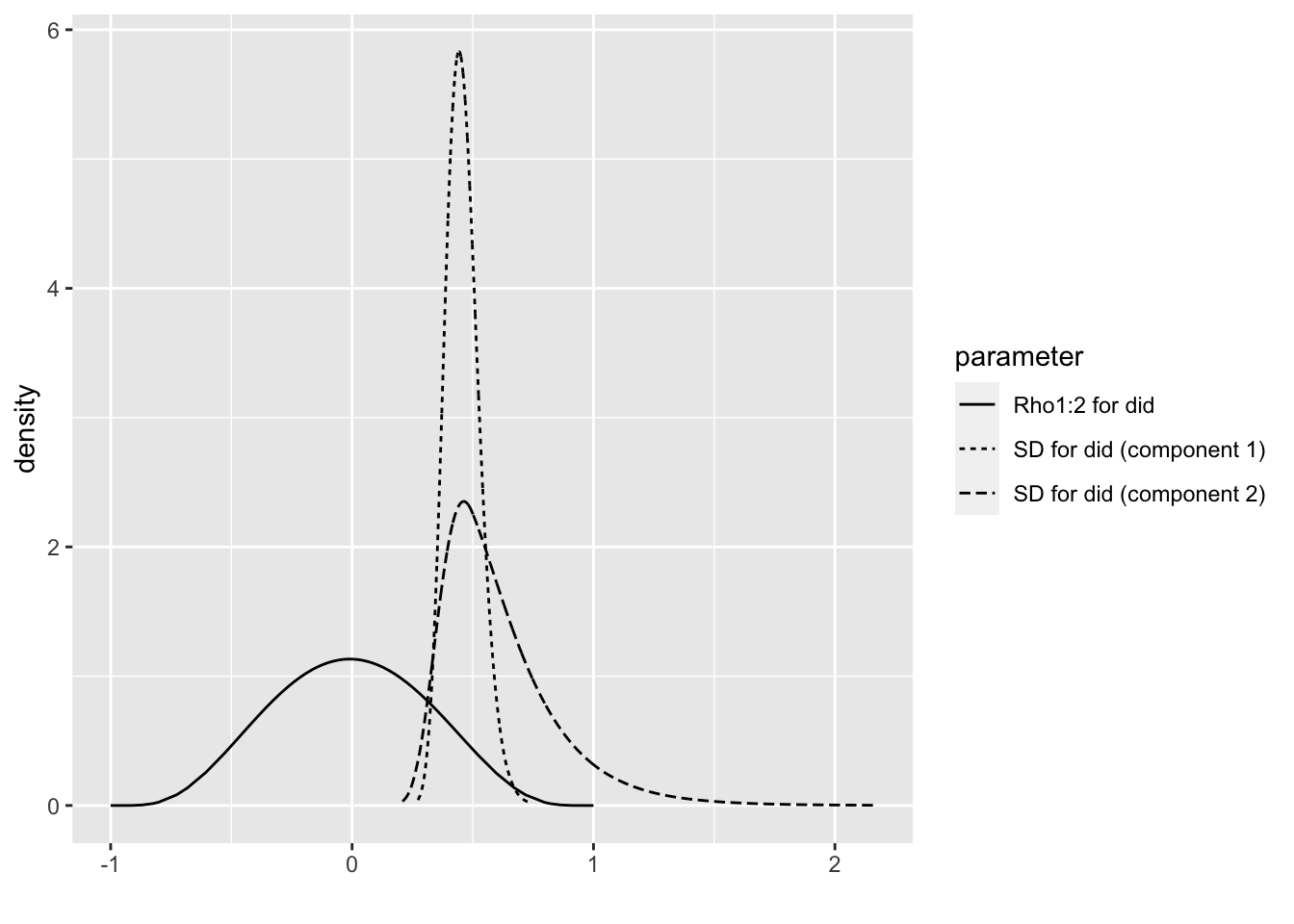
2. data(bangladesh) evaluate the influences on contraceptive use (changing attitudes) of age and number of children
Now consider the predictor variables age.centered and living.children, also contained in data(bangladesh). Suppose that age influences contraceptive use (changing attitudes) and number of children (older people have had more time to have kids). Number of children may also directly influence contraceptive use. Draw a DAG that reflects these hypothetical relationships. Then build models needed to evaluate the DAG. You will need at least two models. Retain district and ur- ban, as in Problem 1. What do you conclude about the causal influence of age and children?
library(dagitty)
hw9.2dag <- dagitty("dag{
C <- A
K <- A
C <- K
}")
plot(hw9.2dag)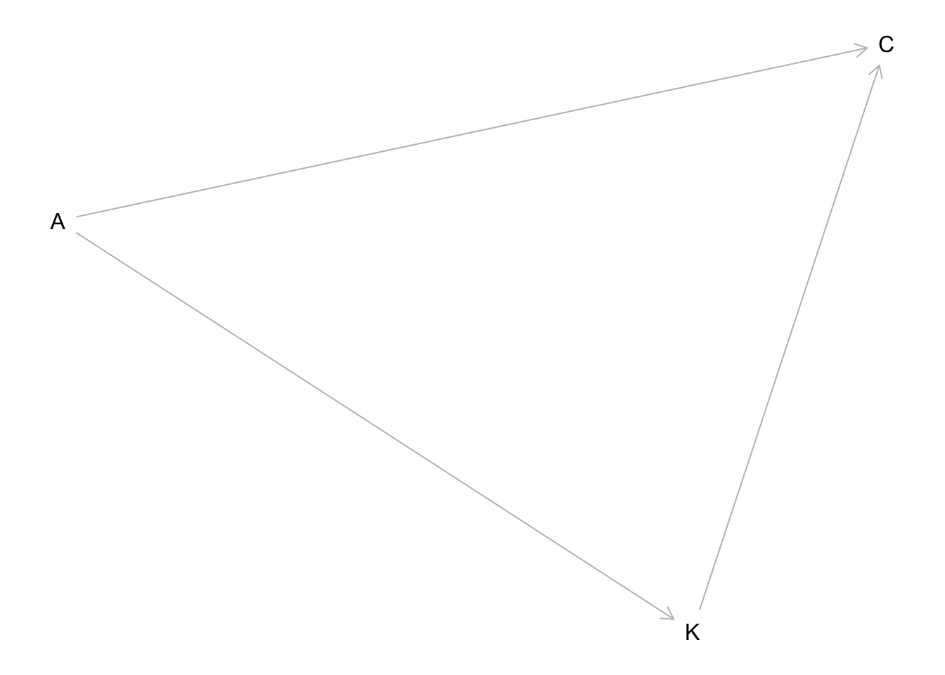 A is age, K is number of children, and C is contraception use.
To study this DAG, we should estimate both the total causal influence of A and then condition also on K and see if the direct influence of A is smaller.
2.1 model for the total influence of A
2.1 rethinking
dat_list$children <- standardize( d$living.children )
dat_list$age <- standardize( d$age.centered )

m2.1 <- ulam( alist(
C ~ bernoulli( p ),
logit(p) <- a[did] + b[did]*urban + bA*age,
c(a,b)[did] ~ multi_normal( c(abar,bbar) , Rho , Sigma ),
abar ~ normal(0,1),
c(bbar,bA) ~ normal(0,0.5),
Rho ~ lkj_corr(2),
Sigma ~ exponential(1)
) , data=dat_list , chains=4 , cores=4 )
## Warning: Bulk Effective Samples Size (ESS) is too low, indicating posterior means and medians may be unreliable.
## Running the chains for more iterations may help. See
## http://mc-stan.org/misc/warnings.html#bulk-ess## Warning: Tail Effective Samples Size (ESS) is too low, indicating posterior variances and tail quantiles may be unreliable.
## Running the chains for more iterations may help. See
## http://mc-stan.org/misc/warnings.html#tail-essprecis(m2.1)## mean sd 5.5% 94.5% n_eff Rhat4
## abar -0.69027935 0.09839765 -0.849204797 -0.5307997 1527.989 1.0000145
## bA 0.08575952 0.04863796 0.006913121 0.1645410 3479.560 0.9992465
## bbar 0.64396667 0.15978274 0.382250689 0.9000550 1186.593 0.9992846precis( m2.1 , depth=3 , pars=c("Rho","Sigma") )## mean sd 5.5% 94.5% n_eff Rhat4
## Rho[1,1] 1.0000000 0.000000e+00 1.0000000 1.0000000 NaN NaN
## Rho[1,2] -0.6628487 1.623307e-01 -0.8727841 -0.3596225 422.4545 1.003141
## Rho[2,1] -0.6628487 1.623307e-01 -0.8727841 -0.3596225 422.4545 1.003141
## Rho[2,2] 1.0000000 5.678775e-17 1.0000000 1.0000000 1800.2697 0.997998
## Sigma[1] 0.5850329 1.000878e-01 0.4320000 0.7481646 546.6285 1.007837
## Sigma[2] 0.7978350 2.034641e-01 0.4883978 1.1375241 246.7951 1.024439In this model, the total causal effect of age is positive and very small. Older individuals use slightly more contraception.
2.1 inla
library(INLA)
library(brinla)


dat_list$children <- standardize( d$living.children )
dat_list$age <- standardize( d$age.centered )


d2.i <- d %>%
  #make a new variable of district that is continuous
  mutate(C = use.contraception,
         did = as.integer( as.factor(d$district)),
         a.did= did,
         b.did= did + max(did),
         children= standardize( living.children ) ,
         age = standardize( age.centered )
  )

n.district= max(d1.i$did) ## = 60


m2.1.i <- inla(C ~ 1+ urban + age + f(a.did, model="iid2d", n= 2*n.district) + f(b.did, urban, copy= "a.did"), data= d2.i, family = "binomial",
              Ntrials = 1,
              control.fixed = list(
        mean= 0,
        prec= 1/(0.5^2),
        mean.intercept= 0,
        prec.intercept= 1
        ),
              control.family = list(control.link=list(model="logit")),
              control.predictor=list(link=1, compute=T),
              control.compute=list(config=T, dic=TRUE, waic= TRUE))
summary(m2.1.i)
##
## Call:
## c("inla(formula = C ~ 1 + urban + age + f(a.did, model = \"iid2d\", ",
## " n = 2 * n.district) + f(b.did, urban, copy = \"a.did\"), family =
## \"binomial\", ", " data = d2.i, Ntrials = 1, control.compute =
## list(config = T, ", " dic = TRUE, waic = TRUE), control.predictor =
## list(link = 1, ", " compute = T), control.family = list(control.link =
## list(model = \"logit\")), ", " control.fixed = list(mean = 0, prec =
## 1/(0.5^2), mean.intercept = 0, ", " prec.intercept = 1))")
## Time used:
## Pre = 1.86, Running = 3.62, Post = 0.376, Total = 5.85
## Fixed effects:
## mean sd 0.025quant 0.5quant 0.975quant mode kld
## (Intercept) -0.689 0.100 -0.887 -0.689 -0.495 -0.688 0
## urban 0.640 0.158 0.331 0.639 0.951 0.639 0
## age 0.084 0.049 -0.012 0.084 0.180 0.084 0
##
## Random effects:
## Name Model
## a.did IID2D model
## b.did Copy
##
## Model hyperparameters:
## mean sd 0.025quant 0.5quant 0.975quant
## Precision for a.did (component 1) 3.088 1.017 1.570 2.930 5.516
## Precision for a.did (component 2) 1.904 0.925 0.703 1.709 4.234
## Rho1:2 for a.did -0.662 0.146 -0.873 -0.687 -0.309
## mode
## Precision for a.did (component 1) 2.640
## Precision for a.did (component 2) 1.384
## Rho1:2 for a.did -0.739
##
## Expected number of effective parameters(stdev): 52.75(5.30)
## Number of equivalent replicates : 36.66
##
## Deviance Information Criterion (DIC) ...............: 2466.13
## Deviance Information Criterion (DIC, saturated) ....: 2466.13
## Effective number of parameters .....................: 53.80
##
## Watanabe-Akaike information criterion (WAIC) ...: 2465.68
## Effective number of parameters .................: 51.57
##
## Marginal log-Likelihood: -1253.38
## Posterior marginals for the linear predictor and
## the fitted values are computedbri.hyperpar.summary(m2.1.i)## mean sd q0.025 q0.5
## SD for a.did (component 1) 0.5912211 0.09440575 0.4264479 0.5840307
## SD for a.did (component 2) 0.7838379 0.17978820 0.4868598 0.7646316
## Rho1:2 for a.did -0.6619113 0.14617008 -0.8730792 -0.6878622
## q0.975 mode
## SD for a.did (component 1) 0.7963088 0.5707599
## SD for a.did (component 2) 1.1895932 0.7281630
## Rho1:2 for a.did -0.3103507 -0.7391103bri.hyperpar.plot(m2.1.i)
the intercept is abar
why didn’t it work using did as an intercept instead of 1?
2.2 model for the direct influence of A (with both K and A)
2.2 rethinking
m2.2 <- ulam( alist(
C ~ bernoulli( p ),
logit(p) <- a[did] + b[did]*urban + bK*children + bA*age,
c(a,b)[did] ~ multi_normal( c(abar,bbar) , Rho , Sigma ),
abar ~ normal(0,1),
c(bbar,bK,bA) ~ normal(0,0.5),
Rho ~ lkj_corr(2),
Sigma ~ exponential(1)
) , data=dat_list , chains=4 , cores=4 )
## Warning: Bulk Effective Samples Size (ESS) is too low, indicating posterior means and medians may be unreliable.
## Running the chains for more iterations may help. See
## http://mc-stan.org/misc/warnings.html#bulk-ess## Warning: Tail Effective Samples Size (ESS) is too low, indicating posterior variances and tail quantiles may be unreliable.
## Running the chains for more iterations may help. See
## http://mc-stan.org/misc/warnings.html#tail-essprecis(m2.2)## mean sd 5.5% 94.5% n_eff Rhat4
## abar -0.7144545 0.10234481 -0.8818230 -0.5521382 1687.773 0.9995983
## bA -0.2612862 0.07138079 -0.3749902 -0.1504531 1743.880 0.9985095
## bK 0.5115326 0.07209485 0.3967871 0.6266893 1737.818 1.0001393
## bbar 0.6888011 0.15762259 0.4408375 0.9414319 1142.356 0.9990996precis( m2.2 , depth=3 , pars=c("Rho","Sigma") )## mean sd 5.5% 94.5% n_eff Rhat4
## Rho[1,1] 1.0000000 0.000000e+00 1.0000000 1.0000000 NaN NaN
## Rho[1,2] -0.6376823 1.708759e-01 -0.8538454 -0.3368814 370.5424 1.002529
## Rho[2,1] -0.6376823 1.708759e-01 -0.8538454 -0.3368814 370.5424 1.002529
## Rho[2,2] 1.0000000 6.153016e-17 1.0000000 1.0000000 1944.3327 0.997998
## Sigma[1] 0.6063893 9.665623e-02 0.4611645 0.7679767 544.1599 1.001116
## Sigma[2] 0.7538359 1.974397e-01 0.4344186 1.0786125 226.6856 1.021838In this model, the direct effect of age is negative, and much farther from zero than before. The effect of number of children is strong and positive. These results are consistent with the DAG, because they imply that the reason the total effect of age, from m2.1, is positive is that older individuals also have more kids. Having more kids increases contraception. Being older, controlling for kids, actually makes con- traception less likely.
2.2 inla
library(INLA)
library(brinla)


m2.2.i <- inla(C ~ 1+ urban + age + children + f(a.did, model="iid2d", n= 2*n.district) + f(b.did, urban, copy= "a.did"), data= d2.i, family = "binomial",
              Ntrials = 1,
              control.fixed = list(
        mean= 0,
        prec= 1/(0.5^2),
        mean.intercept= 0,
        prec.intercept= 1
        ),
              control.family = list(control.link=list(model="logit")),
              control.predictor=list(link=1, compute=T),
              control.compute=list(config=T, dic=TRUE, waic= TRUE))
summary(m2.2.i)
##
## Call:
## c("inla(formula = C ~ 1 + urban + age + children + f(a.did, model =
## \"iid2d\", ", " n = 2 * n.district) + f(b.did, urban, copy =
## \"a.did\"), family = \"binomial\", ", " data = d2.i, Ntrials = 1,
## control.compute = list(config = T, ", " dic = TRUE, waic = TRUE),
## control.predictor = list(link = 1, ", " compute = T), control.family =
## list(control.link = list(model = \"logit\")), ", " control.fixed =
## list(mean = 0, prec = 1/(0.5^2), mean.intercept = 0, ", "
## prec.intercept = 1))")
## Time used:
## Pre = 1.99, Running = 3.13, Post = 0.4, Total = 5.52
## Fixed effects:
## mean sd 0.025quant 0.5quant 0.975quant mode kld
## (Intercept) -0.718 0.103 -0.922 -0.717 -0.516 -0.716 0
## urban 0.693 0.158 0.381 0.693 1.005 0.692 0
## age -0.264 0.070 -0.401 -0.264 -0.128 -0.263 0
## children 0.512 0.071 0.375 0.512 0.652 0.511 0
##
## Random effects:
## Name Model
## a.did IID2D model
## b.did Copy
##
## Model hyperparameters:
## mean sd 0.025quant 0.5quant 0.975quant
## Precision for a.did (component 1) 2.832 0.926 1.449 2.688 5.040
## Precision for a.did (component 2) 1.958 0.968 0.713 1.751 4.401
## Rho1:2 for a.did -0.657 0.148 -0.871 -0.682 -0.299
## mode
## Precision for a.did (component 1) 2.424
## Precision for a.did (component 2) 1.409
## Rho1:2 for a.did -0.734
##
## Expected number of effective parameters(stdev): 54.03(5.28)
## Number of equivalent replicates : 35.79
##
## Deviance Information Criterion (DIC) ...............: 2411.00
## Deviance Information Criterion (DIC, saturated) ....: 2411.00
## Effective number of parameters .....................: 55.02
##
## Watanabe-Akaike information criterion (WAIC) ...: 2410.73
## Effective number of parameters .................: 52.90
##
## Marginal log-Likelihood: -1228.29
## Posterior marginals for the linear predictor and
## the fitted values are computedbri.hyperpar.summary(m2.2.i)## mean sd q0.025 q0.5
## SD for a.did (component 1) 0.6170742 0.0977858 0.4460300 0.6097704
## SD for a.did (component 2) 0.7746153 0.1801363 0.4774009 0.7553064
## Rho1:2 for a.did -0.6566265 0.1479663 -0.8707183 -0.6828040
## q0.975 mode
## SD for a.did (component 1) 0.8291373 0.5965057
## SD for a.did (component 2) 1.1813881 0.7186946
## Rho1:2 for a.did -0.3010549 -0.7346392bri.hyperpar.plot(m2.2.i)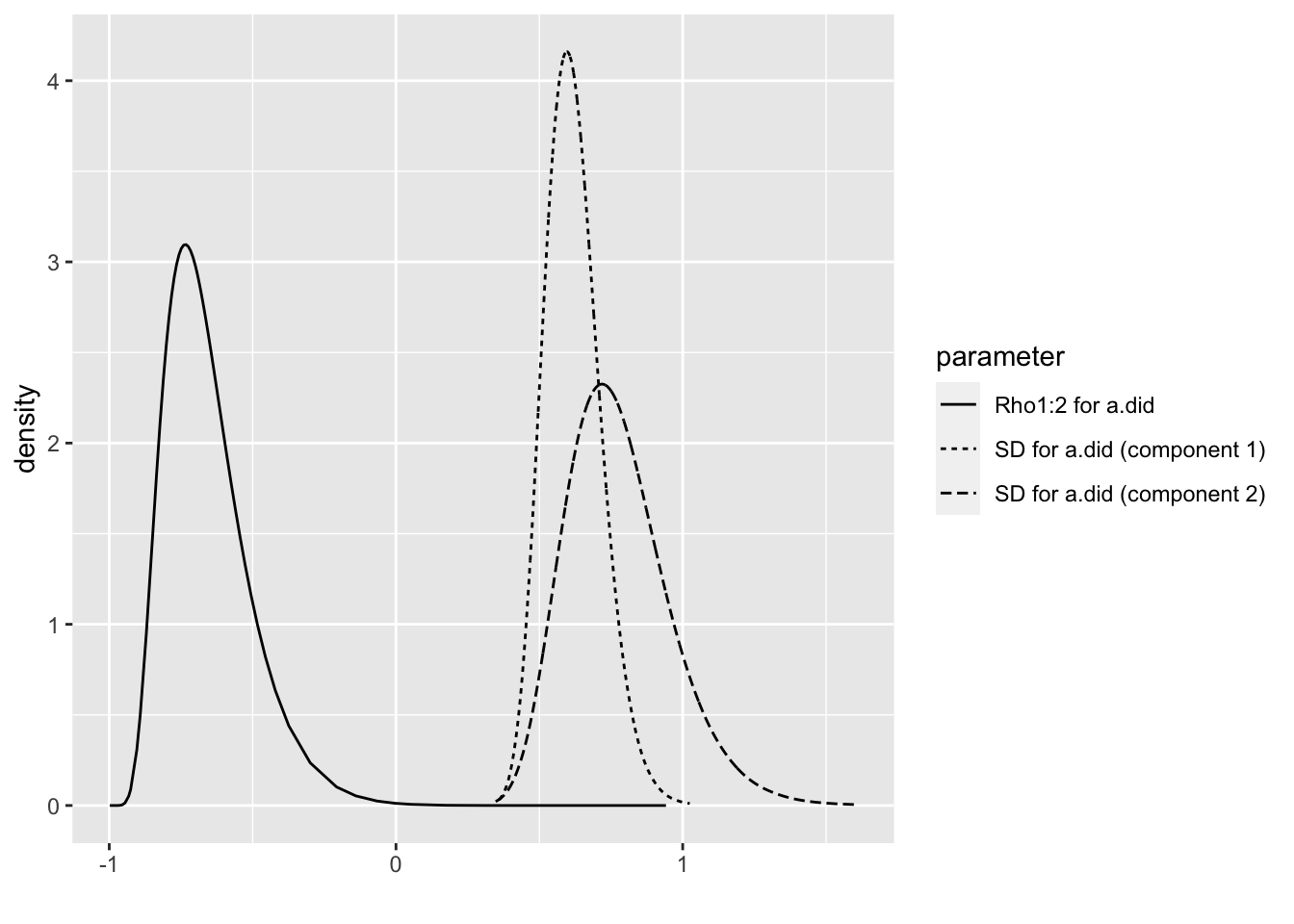
3. data(bangladesh) monotonic ordered category - INCOMPLETE
Modify any models from Problem 2 that contained that children variable and model the variable now as a monotonic ordered category, like education from the week we did ordered categories. Education in that example had 8 categories. Children here will have fewer (no one in the sample had 8 children). So modify the code appropriately. What do you conclude about the causal influence of each additional child on use of contraception?
nope, not doing ordered categories