Statistical Rethinking 2nd edition Homework 8 in INLA
library(tidyverse)
library(rethinking)
library(dagitty)
library(INLA)
library(knitr)
library(stringr)
1. data(reedfrogs) add the predation and size treatment variables to the varying intercepts model
Revisit the Reed frog survival data, data(reedfrogs), and add the predation and size treatment variables to the varying intercepts model. Consider models with either predictor alone, both predictors, as well as a model including their interaction. What do you infer about the causal influence of these predictor variables? Also focus on the inferred variation across tanks (the σ across tanks). Explain why it changes as it does across models with different predictors included.
library(rethinking)
data(reedfrogs)
d <- reedfrogs
1.1 varying intercepts model
Si ∼ Binomial(Ni, pi)
logit(pi) = αtank[i]
αj ∼ Normal(\(\bar{\alpha}\), σ) [adaptive prior]
\(\bar{\alpha}\) ∼ Normal(0, 1.5) [prior for average tank]
σ ∼ Exponential(1) [prior for standard deviation of tanks]
1.1 rethinking
dat <- list(
S = d$surv,
n = d$density,
tank = 1:nrow(d),
pred = ifelse( d$pred=="no" , 0L , 1L ),
size_ = ifelse( d$size=="small" , 1L , 2L )
)
m1.1 <- ulam( alist(
S ~ binomial( n , p ),
logit(p) <- a[tank],
a[tank] ~ normal( a_bar , sigma ),
a_bar ~ normal( 0 , 1.5 ),
sigma ~ exponential( 1 )
), data=dat , chains=4 , cores=4 , log_lik=TRUE )
precis(m1.1, depth= 2)## mean sd 5.5% 94.5% n_eff Rhat4
## a[1] 2.125835347 0.8578613 0.877026178 3.563749653 3574.159 0.9992438
## a[2] 3.079684138 1.0927604 1.543793010 4.987493959 2803.517 1.0003355
## a[3] 0.998984993 0.6602145 -0.002616554 2.105327729 3285.692 0.9999952
## a[4] 3.064522649 1.1112711 1.490482423 4.919059335 2805.443 0.9996481
## a[5] 2.107561809 0.8628401 0.807463604 3.608633785 4216.439 0.9983662
## a[6] 2.152478710 0.8481387 0.883298322 3.612525323 3435.997 0.9985804
## a[7] 3.066007820 1.1290047 1.406274589 5.041585295 2751.904 0.9992932
## a[8] 2.136825865 0.8769736 0.825082001 3.606325004 3168.700 0.9986082
## a[9] -0.163546970 0.6155228 -1.170867407 0.785851060 3564.793 0.9987359
## a[10] 2.131381662 0.8969930 0.840371005 3.645210404 4514.376 0.9982946
## a[11] 0.995764101 0.6863586 -0.023770616 2.128337273 3866.269 0.9986207
## a[12] 0.597490009 0.6306111 -0.402098748 1.627725627 6602.060 0.9990868
## a[13] 1.007182875 0.6895273 -0.045523832 2.172033223 5233.702 0.9987351
## a[14] 0.214788179 0.6071261 -0.751287708 1.190939396 4120.260 0.9984749
## a[15] 2.157834372 0.9260477 0.811490741 3.737503601 4448.907 0.9984093
## a[16] 2.137729788 0.8882259 0.866991838 3.566530914 3760.869 0.9985010
## a[17] 2.899515167 0.7825245 1.796174535 4.231662640 2877.859 0.9997805
## a[18] 2.389794145 0.6889933 1.347420387 3.571609557 3841.997 0.9988757
## a[19] 2.022210350 0.5908458 1.140798783 3.022109553 4758.023 0.9985136
## a[20] 3.657450380 0.9877312 2.230005317 5.316288415 2518.673 0.9987020
## a[21] 2.402766159 0.6570261 1.415850127 3.518011892 3565.431 0.9985523
## a[22] 2.397296830 0.6710211 1.412191316 3.559121326 3146.261 0.9998900
## a[23] 2.393213210 0.6638736 1.406273771 3.525478092 3834.133 0.9985088
## a[24] 1.693588633 0.5149530 0.941144925 2.539002537 2824.197 1.0014749
## a[25] -0.995166068 0.4463296 -1.710755258 -0.301571673 3865.779 0.9996741
## a[26] 0.162507087 0.3919246 -0.461147532 0.794377551 4724.676 0.9983795
## a[27] -1.421878457 0.4895467 -2.236695600 -0.691261117 4591.762 0.9989342
## a[28] -0.465063723 0.3931078 -1.121542150 0.155770523 5584.358 0.9985935
## a[29] 0.153685065 0.3968466 -0.487781910 0.785330016 4286.095 0.9990853
## a[30] 1.444777999 0.5006918 0.666908079 2.281608213 5143.577 0.9987162
## a[31] -0.640577338 0.4095741 -1.306626667 0.019058908 4436.188 0.9983738
## a[32] -0.299330140 0.3979798 -0.954024720 0.318169019 4791.085 0.9992930
## a[33] 3.198113424 0.7862823 2.078694773 4.558195376 3710.493 0.9988089
## a[34] 2.703744414 0.6408673 1.786304026 3.825777848 3306.811 1.0000666
## a[35] 2.674141599 0.5853507 1.827103600 3.681747951 3930.065 0.9993322
## a[36] 2.048243083 0.5044923 1.267909313 2.873675315 4250.835 0.9992327
## a[37] 2.078229728 0.5023080 1.319505918 2.930892831 4286.762 0.9990616
## a[38] 3.904815111 1.0078236 2.448300052 5.603644762 2932.318 0.9997694
## a[39] 2.711671817 0.6477156 1.792607120 3.854934563 2804.334 0.9997096
## a[40] 2.349675427 0.5803703 1.508897970 3.323135839 3321.732 0.9993985
## a[41] -1.811532280 0.4582408 -2.581025536 -1.121977408 3088.732 0.9990591
## a[42] -0.572500363 0.3307254 -1.125966764 -0.053954093 5149.240 0.9983800
## a[43] -0.458986960 0.3386403 -1.017930829 0.079641854 4132.104 0.9997257
## a[44] -0.335625279 0.3518663 -0.907470123 0.230313595 4812.702 0.9984103
## a[45] 0.578520748 0.3423581 0.049808641 1.129395895 4374.925 1.0007021
## a[46] -0.564609960 0.3492258 -1.137926024 -0.009070418 4669.724 0.9991134
## a[47] 2.058256421 0.4848865 1.361180121 2.897531766 4784.677 0.9987961
## a[48] 0.005182228 0.3399494 -0.538240089 0.550960809 4257.455 0.9990758
## a_bar 1.345047407 0.2578896 0.955563652 1.773681340 2854.933 0.9995858
## sigma 1.611566510 0.2125062 1.292106593 1.969722187 1636.190 1.00101681.1 INLA
following example: https://people.bath.ac.uk/jjf23/brinla/reeds.html
Here I’m missing custom priors I’ll use a half cauchy prior for the \(\sigma\) to constrain it to >0 numbers, which is what the exponential does as well.
library(brinla)
library(INLA)

d1.i <- d %>%
  mutate(tank = row_number(),
         pred.no= na_if(if_else(pred=="no", 1, 0), 0),
         pred.yes= na_if(if_else(pred=="pred", 1, 0), 0),
         size.small= na_if(if_else(size=="small", 1, 0), 0),
         size.big= na_if(if_else(size=="big", 1, 0), 0)
         )

# number of trials is d1.i$density

halfcauchy = "expression:
              lambda = 0.022;
              precision = exp(log_precision);
              logdens = -1.5*log_precision-log(pi*lambda)-log(1+1/(precision*lambda^2));
              log_jacobian = log_precision;
              return(logdens+log_jacobian);"

hcprior = list(prec = list(prior = halfcauchy))

m1.1.i <- inla(surv ~ 1 + f(tank, model="iid", hyper = hcprior), data= d1.i, family = "binomial",
              Ntrials = density,
              control.family = list(control.link=list(model="logit")),
              control.predictor=list(link=1, compute=T),
              control.compute=list(config=T, dic=TRUE, waic= TRUE))
summary(m1.1.i)
##
## Call:
## c("inla(formula = surv ~ 1 + f(tank, model = \"iid\", hyper = hcprior),
## ", " family = \"binomial\", data = d1.i, Ntrials = density,
## control.compute = list(config = T, ", " dic = TRUE, waic = TRUE),
## control.predictor = list(link = 1, ", " compute = T), control.family =
## list(control.link = list(model = \"logit\")))" )
## Time used:
## Pre = 1.51, Running = 0.205, Post = 0.203, Total = 1.91
## Fixed effects:
## mean sd 0.025quant 0.5quant 0.975quant mode kld
## (Intercept) 1.38 0.256 0.89 1.375 1.901 1.364 0
##
## Random effects:
## Name Model
## tank IID model
##
## Model hyperparameters:
## mean sd 0.025quant 0.5quant 0.975quant mode
## Precision for tank 0.415 0.109 0.237 0.404 0.661 0.381
##
## Expected number of effective parameters(stdev): 40.36(1.26)
## Number of equivalent replicates : 1.19
##
## Deviance Information Criterion (DIC) ...............: 214.00
## Deviance Information Criterion (DIC, saturated) ....: 89.62
## Effective number of parameters .....................: 39.50
##
## Watanabe-Akaike information criterion (WAIC) ...: 205.61
## Effective number of parameters .................: 22.72
##
## Marginal log-Likelihood: -140.19
## Posterior marginals for the linear predictor and
## the fitted values are computedm1.1.i$summary.fixed## mean sd 0.025quant 0.5quant 0.975quant mode
## (Intercept) 1.380249 0.2562768 0.8904279 1.374944 1.90069 1.364469
## kld
## (Intercept) 1.902443e-05m1.1.i$summary.hyperpar## mean sd 0.025quant 0.5quant 0.975quant
## Precision for tank 0.4152469 0.1088217 0.2366839 0.4035007 0.6608823
## mode
## Precision for tank 0.3807222bri.hyperpar.summary(m1.1.i)## mean sd q0.025 q0.5 q0.975 mode
## SD for tank 1.59197 0.2096781 1.231084 1.573964 2.053666 1.539229it looks like the intercept mean and sd correspond to the \(\bar{\alpha}\) mean and sd, and the SD for tank corresponds to the \(\sigma\). this makes sense, because the \(\bar{\alpha}\) is the average baseline survival for all the tadpoles, which is what the intercept is. BUT I WOULD LOVE IF SOMEONE ELSE CONFIRMED THIS INTERPRETATION.
1.2 varying intercepts + predation
Si ∼ Binomial(Ni, pi)
logit(pi) = αtank[i] + \(\beta\)[pred]
\(\beta\)∼ Normal(-0.5,1)
αj ∼ Normal(\(\bar{\alpha}\), σ) [adaptive prior]
\(\bar{\alpha}\) ∼ Normal(0, 1.5) [prior for average tank]
σ ∼ Exponential(1) [prior for standard deviation of tanks]
1.2 rethinking
# pred
m1.2 <- ulam(
alist(
S ~ binomial( n , p ),
logit(p) <- a[tank] + bp*pred,
a[tank] ~ normal( a_bar , sigma ),
bp ~ normal( -0.5 , 1 ),
a_bar ~ normal( 0 , 1.5 ),
sigma ~ exponential( 1 )
), data=dat , chains=4 , cores=4 , log_lik=TRUE )
## Warning: Bulk Effective Samples Size (ESS) is too low, indicating posterior means and medians may be unreliable.
## Running the chains for more iterations may help. See
## http://mc-stan.org/misc/warnings.html#bulk-essprecis(m1.2)## mean sd 5.5% 94.5% n_eff Rhat4
## bp -2.4430629 0.2998946 -2.9060742 -1.958471 168.7359 1.005689
## a_bar 2.5415598 0.2337773 2.1714476 2.922271 199.9063 1.006978
## sigma 0.8271075 0.1466172 0.5999589 1.070372 572.1093 1.0020241.2 inla
library(brinla)
library(INLA)

# number of trials is d1.i$density

halfcauchy = "expression:
              lambda = 0.022;
              precision = exp(log_precision);
              logdens = -1.5*log_precision-log(pi*lambda)-log(1+1/(precision*lambda^2));
              log_jacobian = log_precision;
              return(logdens+log_jacobian);"

hcprior = list(prec = list(prior = halfcauchy))

m1.2.i <- inla(surv ~ 1 + pred + f(tank, model="iid", hyper = hcprior), data= d1.i, family = "binomial",
              Ntrials = density,
              control.fixed = list(
        mean= -0.5,
        prec= 1,
        mean.intercept= 0,
        prec.intercept= 1/(1.5^2)),
              control.family = list(control.link=list(model="logit")),
              control.predictor=list(link=1, compute=T),
              control.compute=list(config=T, dic=TRUE, waic= TRUE))
summary(m1.2.i)
##
## Call:
## c("inla(formula = surv ~ 1 + pred + f(tank, model = \"iid\", hyper =
## hcprior), ", " family = \"binomial\", data = d1.i, Ntrials = density,
## control.compute = list(config = T, ", " dic = TRUE, waic = TRUE),
## control.predictor = list(link = 1, ", " compute = T), control.family =
## list(control.link = list(model = \"logit\")), ", " control.fixed =
## list(mean = -0.5, prec = 1, mean.intercept = 0, ", " prec.intercept =
## 1/(1.5^2)))")
## Time used:
## Pre = 1.43, Running = 0.197, Post = 0.201, Total = 1.83
## Fixed effects:
## mean sd 0.025quant 0.5quant 0.975quant mode kld
## (Intercept) 2.523 0.225 2.088 2.520 2.974 2.515 0
## predpred -2.435 0.288 -2.997 -2.437 -1.863 -2.440 0
##
## Random effects:
## Name Model
## tank IID model
##
## Model hyperparameters:
## mean sd 0.025quant 0.5quant 0.975quant mode
## Precision for tank 1.80 0.677 0.85 1.68 3.46 1.48
##
## Expected number of effective parameters(stdev): 28.98(3.36)
## Number of equivalent replicates : 1.66
##
## Deviance Information Criterion (DIC) ...............: 204.42
## Deviance Information Criterion (DIC, saturated) ....: 79.99
## Effective number of parameters .....................: 29.04
##
## Watanabe-Akaike information criterion (WAIC) ...: 201.45
## Effective number of parameters .................: 19.59
##
## Marginal log-Likelihood: -122.10
## Posterior marginals for the linear predictor and
## the fitted values are computedm1.2.i$summary.fixed## mean sd 0.025quant 0.5quant 0.975quant mode
## (Intercept) 2.523164 0.2252490 2.087742 2.520414 2.974171 2.514827
## predpred -2.435197 0.2876891 -2.996768 -2.437046 -1.863173 -2.440294
## kld
## (Intercept) 2.391528e-07
## predpred 8.877976e-07bri.hyperpar.summary(m1.2.i)## mean sd q0.025 q0.5 q0.975 mode
## SD for tank 0.7815832 0.1385647 0.5384615 0.7711308 1.082806 0.75176251.3 varying intercepts + size
Si ∼ Binomial(Ni, pi)
logit(pi) = αtank[i] + \(\beta\)size
\(\beta\)∼ Normal(0 , 0.5 ) αj ∼ Normal(\(\bar{\alpha}\), σ) [adaptive prior]
\(\bar{\alpha}\) ∼ Normal(0, 1.5) [prior for average tank]
σ ∼ Exponential(1) [prior for standard deviation of tanks]
1.3 rethinking
library(rethinking)
data(reedfrogs)
d <- reedfrogs

# size
m1.3 <- ulam( alist(
S ~ binomial( n , p ),
logit(p) <- a[tank] + s[size_],
a[tank] ~ normal( a_bar , sigma ),
s[size_] ~ normal( 0 , 0.5 ),
a_bar ~ normal( 0 , 1.5 ),
sigma ~ exponential( 1 )
), data=dat , chains=4 , cores=4 , log_lik=TRUE )
## Warning: Bulk Effective Samples Size (ESS) is too low, indicating posterior means and medians may be unreliable.
## Running the chains for more iterations may help. See
## http://mc-stan.org/misc/warnings.html#bulk-ess## Warning: Tail Effective Samples Size (ESS) is too low, indicating posterior variances and tail quantiles may be unreliable.
## Running the chains for more iterations may help. See
## http://mc-stan.org/misc/warnings.html#tail-essprecis(m1.3, depth=2)## mean sd 5.5% 94.5% n_eff Rhat4
## a[1] 2.17345207 0.9319950 0.7761505 3.67423844 499.6435 1.0004651
## a[2] 3.09970098 1.1627310 1.3753649 5.05207425 819.8692 0.9999842
## a[3] 1.07262815 0.8039234 -0.1562473 2.34707211 509.3498 1.0005668
## a[4] 3.10980987 1.1523957 1.4143631 5.09648713 593.5731 1.0000390
## a[5] 1.97495079 0.9955697 0.4901889 3.63823208 664.3093 1.0025344
## a[6] 1.93729202 0.9480752 0.5217026 3.48318191 675.5431 1.0058596
## a[7] 2.90960252 1.1690395 1.1880459 4.87074861 808.0568 1.0035432
## a[8] 1.93881563 0.9567468 0.4989728 3.51846638 712.0215 1.0047067
## a[9] -0.10003953 0.7528785 -1.2807865 1.10980141 354.4239 1.0038207
## a[10] 2.18746650 0.9797261 0.7375766 3.82684201 603.0839 1.0001781
## a[11] 1.06000144 0.8040228 -0.2010947 2.35159965 330.4173 1.0051495
## a[12] 0.65008431 0.7323813 -0.4709883 1.76731364 386.1692 1.0058628
## a[13] 0.81457273 0.7749713 -0.3911966 2.05704403 349.9527 1.0094325
## a[14] -0.02536241 0.7202389 -1.1688180 1.10779848 400.8156 1.0058498
## a[15] 1.97173561 0.9731446 0.5531756 3.64536989 767.6827 1.0037847
## a[16] 1.94833370 0.9886317 0.4341261 3.60893143 554.9555 1.0027725
## a[17] 2.94990006 0.8634043 1.6458344 4.42307444 477.4091 0.9993947
## a[18] 2.46694180 0.7575293 1.3115983 3.72705463 454.7485 1.0031795
## a[19] 2.08483075 0.7218820 0.9249065 3.26710863 379.1938 1.0013284
## a[20] 3.71688703 1.0921352 2.0873194 5.49231036 662.6515 1.0013400
## a[21] 2.19711491 0.7871551 0.9769018 3.52929636 354.3215 1.0081693
## a[22] 2.17568987 0.7591930 0.9618530 3.40172521 456.3442 1.0039101
## a[23] 2.17446667 0.7857587 0.9658257 3.46641907 522.7335 1.0056787
## a[24] 1.48120228 0.6679605 0.3868568 2.55304266 368.3295 1.0052565
## a[25] -0.91361951 0.6005678 -1.8452812 0.05972356 233.3428 1.0052000
## a[26] 0.23871034 0.5786945 -0.6758760 1.16226175 226.6733 1.0027602
## a[27] -1.34433388 0.6261157 -2.3374725 -0.34274145 383.4352 1.0012125
## a[28] -0.38440516 0.5765461 -1.2804852 0.59449993 213.1866 1.0074524
## a[29] -0.06690000 0.5636537 -0.9786765 0.82600700 322.1258 1.0059886
## a[30] 1.22943653 0.6558065 0.2190195 2.28132588 371.2962 1.0055268
## a[31] -0.86930933 0.5844135 -1.8048252 0.09235445 298.9714 1.0068062
## a[32] -0.53715913 0.5616748 -1.4292025 0.34072591 307.6465 1.0092188
## a[33] 3.28667827 0.9113625 1.9152245 4.83344956 403.9710 1.0001905
## a[34] 2.76949771 0.7605488 1.6456121 4.02651831 466.5024 1.0015633
## a[35] 2.79526105 0.7505859 1.6525389 3.99384128 422.5288 1.0026386
## a[36] 2.13515044 0.6476965 1.1368507 3.22215553 253.2498 1.0016715
## a[37] 1.84251525 0.6513578 0.8176832 2.91112834 366.6667 1.0067035
## a[38] 3.72666330 1.0514232 2.1716924 5.51250053 769.2609 0.9996279
## a[39] 2.49120520 0.7613700 1.3403330 3.75929069 452.9642 1.0032631
## a[40] 2.15052083 0.7191019 1.0528257 3.36184577 451.8371 1.0093305
## a[41] -1.73297669 0.6427383 -2.7851721 -0.69444311 262.0498 1.0051869
## a[42] -0.47607488 0.5422143 -1.3230082 0.39346202 208.9523 1.0053384
## a[43] -0.37855967 0.5357837 -1.2175354 0.49661655 213.7359 1.0052193
## a[44] -0.24788702 0.5331680 -1.0898412 0.64869050 192.5527 1.0055149
## a[45] 0.35558976 0.5324301 -0.5087165 1.19619384 269.3661 1.0094972
## a[46] -0.79251852 0.5285400 -1.6493505 0.04958823 242.8992 1.0081172
## a[47] 1.86633354 0.6684197 0.8251676 2.93754201 405.1957 1.0031056
## a[48] -0.21864384 0.5273078 -1.0811366 0.64800617 254.3662 1.0089770
## s[1] 0.23426594 0.4129964 -0.4137626 0.91318408 153.8224 1.0136855
## s[2] -0.08884360 0.4205315 -0.7843759 0.56613030 135.9180 1.0071035
## a_bar 1.28172242 0.4363755 0.5865873 2.00173422 149.8571 1.0081431
## sigma 1.61566009 0.2111806 1.3132128 1.98016979 792.8415 1.00106321.3 inla
library(brinla)
library(INLA)
library(tidyverse)

d1.i <- d %>%
  mutate(tank = row_number(),
         pred.no= na_if(if_else(pred=="no", 1, 0), 0),
         pred.yes= na_if(if_else(pred=="pred", 1, 0), 0),
         size.small= na_if(if_else(size=="small", 1, 0), 0),
         size.big= na_if(if_else(size=="big", 1, 0), 0)
         )

# number of trials is d1.i$density

halfcauchy = "expression:
              lambda = 0.022;
              precision = exp(log_precision);
              logdens = -1.5*log_precision-log(pi*lambda)-log(1+1/(precision*lambda^2));
              log_jacobian = log_precision;
              return(logdens+log_jacobian);"

hcprior = list(prec = list(prior = halfcauchy))

m1.3.i <- inla(surv ~ 1 + size.small+ size.big + f(tank, model="iid", hyper = hcprior), data= d1.i, family = "binomial",
              Ntrials = density,
              control.fixed = list(
        mean= 0,
        prec= 1/(0.5^2),
        mean.intercept= 0,
        prec.intercept= 1/(1.5^2)),
              control.family = list(control.link=list(model="logit")),
              control.predictor=list(link=1, compute=T),
              control.compute=list(config=T, dic=TRUE, waic= TRUE))
summary(m1.3.i)
##
## Call:
## c("inla(formula = surv ~ 1 + size.small + size.big + f(tank, model =
## \"iid\", ", " hyper = hcprior), family = \"binomial\", data = d1.i,
## Ntrials = density, ", " control.compute = list(config = T, dic = TRUE,
## waic = TRUE), ", " control.predictor = list(link = 1, compute = T),
## control.family = list(control.link = list(model = \"logit\")), ", "
## control.fixed = list(mean = 0, prec = 1/(0.5^2), mean.intercept = 0, ",
## " prec.intercept = 1/(1.5^2)))")
## Time used:
## Pre = 1.43, Running = 0.182, Post = 0.23, Total = 1.84
## Fixed effects:
## mean sd 0.025quant 0.5quant 0.975quant mode kld
## (Intercept) 1.272 0.418 0.455 1.271 2.095 1.268 0
## size.small 0.222 0.400 -0.564 0.223 1.007 0.223 0
## size.big -0.081 0.400 -0.866 -0.082 0.705 -0.082 0
##
## Random effects:
## Name Model
## tank IID model
##
## Model hyperparameters:
## mean sd 0.025quant 0.5quant 0.975quant mode
## Precision for tank 0.421 0.111 0.239 0.408 0.672 0.385
##
## Expected number of effective parameters(stdev): 40.42(1.26)
## Number of equivalent replicates : 1.19
##
## Deviance Information Criterion (DIC) ...............: 214.43
## Deviance Information Criterion (DIC, saturated) ....: 90.04
## Effective number of parameters .....................: 39.58
##
## Watanabe-Akaike information criterion (WAIC) ...: 206.21
## Effective number of parameters .................: 22.90
##
## Marginal log-Likelihood: -142.21
## Posterior marginals for the linear predictor and
## the fitted values are computedm1.3.i$summary.fixed## mean sd 0.025quant 0.5quant 0.975quant mode
## (Intercept) 1.27186665 0.4177740 0.4549238 1.27059867 2.095210 1.2681232
## size.small 0.22245891 0.4001376 -0.5640040 0.22269633 1.006898 0.2232035
## size.big -0.08147702 0.4002655 -0.8664804 -0.08182627 0.704788 -0.0824901
## kld
## (Intercept) 2.406671e-06
## size.small 1.123068e-07
## size.big 6.786554e-07bri.hyperpar.summary(m1.3.i)## mean sd q0.025 q0.5 q0.975 mode
## SD for tank 1.582503 0.2100774 1.220948 1.56446 2.045071 1.5296351.4 varying intercepts + predation + size
Si ∼ Binomial(Ni, pi)
logit(pi) = αtank[i] + \(\beta\)size + \(\gamma\)size
\(\gamma\) ∼ Normal(0 , 0.5)
\(\beta\) ∼ Normal(-0.5,1) αj ∼ Normal(\(\bar{\alpha}\), σ) [adaptive prior]
\(\bar{\alpha}\) ∼ Normal(0, 1.5) [prior for average tank]
σ ∼ Exponential(1) [prior for standard deviation of tanks]
1.4 rethinking
# pred + size
m1.4 <- ulam(
alist(
S ~ binomial( n , p ),
logit(p) <- a[tank] + bp*pred + s[size_],
a[tank] ~ normal( a_bar , sigma ),
bp ~ normal( -0.5 , 1 ),
s[size_] ~ normal( 0 , 0.5 ),
a_bar ~ normal( 0 , 1.5 ),
sigma ~ exponential( 1 )
), data=dat , chains=4 , cores=4 , log_lik=TRUE )
## Warning: Bulk Effective Samples Size (ESS) is too low, indicating posterior means and medians may be unreliable.
## Running the chains for more iterations may help. See
## http://mc-stan.org/misc/warnings.html#bulk-essprecis(m1.4, depth=2)## mean sd 5.5% 94.5% n_eff Rhat4
## a[1] 2.4237883 0.7348593 1.28673082 3.6225789 432.9727 1.001936
## a[2] 2.8275702 0.7623963 1.63600941 4.0346942 529.0491 1.005197
## a[3] 1.6904880 0.7186689 0.60970560 2.8620838 413.4064 1.005549
## a[4] 2.8567395 0.7812660 1.63270104 4.1416744 416.5653 1.006153
## a[5] 2.2924183 0.7600521 1.12040918 3.5003247 515.8187 1.003971
## a[6] 2.2890945 0.7456236 1.13398326 3.4873405 494.5496 1.001211
## a[7] 2.7529554 0.8197108 1.56160579 4.1101834 508.5259 1.003351
## a[8] 2.3060100 0.7643283 1.09833845 3.4942726 428.3401 1.006175
## a[9] 2.2239552 0.6805941 1.11013046 3.3244542 303.6484 1.010388
## a[10] 3.5226856 0.7057307 2.43711458 4.6968707 252.2916 1.011289
## a[11] 2.9759071 0.6849384 1.91514527 4.1068925 281.3213 1.005638
## a[12] 2.7255892 0.6560724 1.67170664 3.8110887 303.4140 1.008832
## a[13] 2.7464775 0.6784512 1.67822983 3.8498211 302.9607 1.008885
## a[14] 2.2271624 0.6614753 1.21510633 3.3192970 250.3940 1.010253
## a[15] 3.2858217 0.6822474 2.24250482 4.3858950 288.6834 1.009536
## a[16] 3.2992377 0.6995637 2.20855816 4.4741681 291.1126 1.008619
## a[17] 2.8313090 0.6914988 1.81238554 3.9895034 354.0481 1.003879
## a[18] 2.5415571 0.6631672 1.51529392 3.6149735 373.9830 1.009346
## a[19] 2.2632750 0.6522951 1.28169441 3.3712096 430.9508 1.006780
## a[20] 3.2062378 0.7349194 2.09521552 4.3986330 388.1240 1.011504
## a[21] 2.2983078 0.6619077 1.24321201 3.3638764 410.6148 1.006957
## a[22] 2.3080976 0.6682041 1.28220891 3.4526263 443.0228 1.004005
## a[23] 2.3248635 0.6519924 1.33031283 3.3708382 390.0172 1.010234
## a[24] 1.7720524 0.6173318 0.79421157 2.7826668 418.1520 1.002946
## a[25] 1.6149423 0.6062522 0.66934189 2.5964064 224.7619 1.010043
## a[26] 2.5712509 0.5881656 1.68046491 3.5785654 231.6253 1.012682
## a[27] 1.3008374 0.6273264 0.26986649 2.2931373 235.1511 1.009649
## a[28] 2.0341474 0.5962279 1.09082179 2.9663634 229.1667 1.010822
## a[29] 2.2229945 0.5790097 1.27040676 3.1317319 211.7161 1.009234
## a[30] 3.2134421 0.6046327 2.26197720 4.1934021 200.9597 1.018173
## a[31] 1.5773007 0.5936973 0.60107722 2.4971323 242.1822 1.007159
## a[32] 1.8383147 0.5851350 0.90311890 2.7831585 223.9384 1.009698
## a[33] 3.0451365 0.6687317 1.98662249 4.1406406 424.8942 1.005312
## a[34] 2.7415700 0.6504509 1.73592539 3.7846889 326.9896 1.008532
## a[35] 2.7382008 0.6275698 1.77983739 3.7736569 330.0808 1.009961
## a[36] 2.2904486 0.6048694 1.37065176 3.2802002 405.1218 1.007962
## a[37] 2.0205946 0.6056905 1.07186224 3.0205732 354.1018 1.007331
## a[38] 3.1745632 0.7353991 2.05552167 4.4141523 475.3301 1.003975
## a[39] 2.5068795 0.6362496 1.53529251 3.5723671 335.3820 1.010138
## a[40] 2.2525528 0.6190753 1.27673054 3.2440690 431.4400 1.004211
## a[41] 0.9988831 0.6124238 0.02717937 1.9439021 236.2956 1.011534
## a[42] 1.9517041 0.5650305 1.07914994 2.9011794 191.7744 1.013619
## a[43] 2.0535703 0.5677752 1.16486862 2.9862846 181.5795 1.016140
## a[44] 2.1480760 0.5527467 1.25535208 3.0271480 193.7791 1.014759
## a[45] 2.5906122 0.5537153 1.71895610 3.4978115 204.0346 1.010718
## a[46] 1.6001826 0.5466200 0.73123212 2.4764172 192.3499 1.012209
## a[47] 3.6952600 0.5950642 2.75761084 4.6605961 201.2483 1.014491
## a[48] 2.1046366 0.5490831 1.26142476 2.9699215 193.8766 1.009388
## bp -2.4348637 0.2962117 -2.88552117 -1.9495603 387.3076 1.008328
## s[1] 0.3391476 0.3694226 -0.26579531 0.9178127 183.6084 1.017996
## s[2] -0.0953497 0.3771795 -0.67986336 0.5043115 182.1927 1.017138
## a_bar 2.4053442 0.4091662 1.76155558 3.0883690 127.1681 1.024072
## sigma 0.7890657 0.1432128 0.58570095 1.0379255 526.0016 1.0049831.4 inla
library(brinla)
library(INLA)

# number of trials is d1.i$density

halfcauchy = "expression:
              lambda = 0.022;
              precision = exp(log_precision);
              logdens = -1.5*log_precision-log(pi*lambda)-log(1+1/(precision*lambda^2));
              log_jacobian = log_precision;
              return(logdens+log_jacobian);"

hcprior = list(prec = list(prior = halfcauchy))

m1.4.i <- inla(surv ~ 1 + pred + size.small+ size.big + f(tank, model="iid", hyper = hcprior), data= d1.i, family = "binomial",
              Ntrials = density,
              control.fixed = list(
        mean= list(pred= -0.5,size.small= 0, size.big= 0 ),
        prec= list(pred= 1,size.small= 1, size.big= 1 ),
        mean.intercept= 0,
        prec.intercept= 1/(1.5^2)),
              control.family = list(control.link=list(model="logit")),
              control.predictor=list(link=1, compute=T),
              control.compute=list(config=T, dic=TRUE, waic= TRUE))
summary(m1.4.i)
##
## Call:
## c("inla(formula = surv ~ 1 + pred + size.small + size.big + f(tank, ",
## " model = \"iid\", hyper = hcprior), family = \"binomial\", data =
## d1.i, ", " Ntrials = density, control.compute = list(config = T, dic =
## TRUE, ", " waic = TRUE), control.predictor = list(link = 1, compute =
## T), ", " control.family = list(control.link = list(model = \"logit\")),
## ", " control.fixed = list(mean = list(pred = -0.5, size.small = 0, ", "
## size.big = 0), prec = list(pred = 1, size.small = 1, ", " size.big =
## 1), mean.intercept = 0, prec.intercept = 1/(1.5^2)))" )
## Time used:
## Pre = 1.6, Running = 0.186, Post = 0.264, Total = 2.05
## Fixed effects:
## mean sd 0.025quant 0.5quant 0.975quant mode kld
## (Intercept) 2.161 0.666 0.854 2.161 3.469 2.160 0
## predpred -2.628 0.290 -3.204 -2.626 -2.062 -2.622 0
## size.small 0.729 0.656 -0.559 0.729 2.016 0.729 0
## size.big 0.231 0.656 -1.056 0.231 1.517 0.231 0
##
## Random effects:
## Name Model
## tank IID model
##
## Model hyperparameters:
## mean sd 0.025quant 0.5quant 0.975quant mode
## Precision for tank 2.13 0.907 0.941 1.95 4.40 1.66
##
## Expected number of effective parameters(stdev): 27.66(3.70)
## Number of equivalent replicates : 1.74
##
## Deviance Information Criterion (DIC) ...............: 204.82
## Deviance Information Criterion (DIC, saturated) ....: 80.44
## Effective number of parameters .....................: 27.99
##
## Watanabe-Akaike information criterion (WAIC) ...: 202.79
## Effective number of parameters .................: 19.63
##
## Marginal log-Likelihood: -123.31
## Posterior marginals for the linear predictor and
## the fitted values are computedm1.4.i$summary.fixed## mean sd 0.025quant 0.5quant 0.975quant mode
## (Intercept) 2.1613253 0.6663035 0.8539924 2.1610031 3.469238 2.1604153
## predpred -2.6276156 0.2895818 -3.2042666 -2.6256993 -2.062158 -2.6218552
## size.small 0.7293355 0.6560320 -0.5587394 0.7293248 2.016310 0.7293579
## size.big 0.2308486 0.6557372 -1.0562819 0.2307203 1.517498 0.2305195
## kld
## (Intercept) 1.094653e-07
## predpred 3.292691e-06
## size.small 4.990355e-07
## size.big 1.043209e-08bri.hyperpar.summary(m1.4.i)## mean sd q0.025 q0.5 q0.975 mode
## SD for tank 0.7260825 0.1402651 0.4772367 0.7163201 1.028863 0.69861021.5 varying intercepts + predation + size + predation*size
Si ∼ Binomial(Ni, pi)
this formula’s wrong
logit(pi) = αtank[i] + \(\beta\)predation + \(\gamma\)size + \(\eta\)size*predation
\(\gamma\) ∼ Normal(0 , 0.5) \(\beta\) ∼ Normal(-0.5,1) αj ∼ Normal(\(\bar{\alpha}\), σ) [adaptive prior]
\(\bar{\alpha}\) ∼ Normal(0, 1.5) [prior for average tank] σ ∼ Exponential(1) [prior for standard deviation of tanks]
1.5 rethinking
# pred + size + interaction
m1.5 <- ulam(
alist(
S ~ binomial( n , p),
logit(p) <- a_bar + z[tank]*sigma + s[size_]+ bp[size_]*pred ,
z[tank] ~ normal( 0, 1),
bp[size_] ~ normal(-0.5,1),
s[size_] ~ normal( 0 , 0.5 ),
a_bar ~ normal( 0 , 1.5 ),
sigma ~ exponential( 1 )
), data=dat , chains=4 , cores=4 , log_lik=TRUE )


precis(m1.5, depth=2)
## mean sd 5.5% 94.5% n_eff Rhat4
## z[1] -0.03447354 0.7947785 -1.2479850 1.22693025 2487.5246 0.9988316
## z[2] 0.49272170 0.8939910 -0.9082640 1.93172763 3125.9808 0.9989238
## z[3] -0.94782594 0.8012038 -2.1956580 0.43121579 2596.5411 0.9985249
## z[4] 0.48205490 0.9041177 -0.9477907 1.92946370 3119.6237 0.9987591
## z[5] -0.05018335 0.8370162 -1.3924780 1.32091736 2833.2300 1.0000993
## z[6] -0.00359632 0.8416464 -1.3355377 1.35269373 2169.8957 1.0001977
## z[7] 0.49791174 0.8748225 -0.8451802 1.95348055 2460.6786 0.9990520
## z[8] -0.02530060 0.8067085 -1.3159048 1.29269838 2813.1734 0.9990143
## z[9] -0.08525639 0.6839497 -1.1605948 0.98666760 2152.7093 0.9987845
## z[10] 1.52113860 0.7364583 0.3541629 2.72271453 2274.5354 0.9993257
## z[11] 0.87094206 0.7284642 -0.2777531 2.06757078 2872.5663 1.0017177
## z[12] 0.53487421 0.6963334 -0.5772034 1.66080564 2438.6267 0.9990414
## z[13] 0.24570758 0.7119168 -0.8622668 1.41101751 2478.6887 0.9993966
## z[14] -0.44976131 0.6930189 -1.5507728 0.64838642 2733.0385 0.9984444
## z[15] 0.94958419 0.7438065 -0.2059181 2.19569920 2367.4429 0.9986785
## z[16] 0.95302522 0.7254713 -0.1981445 2.13825080 3193.2469 0.9997914
## z[17] 0.47189535 0.7640470 -0.6991305 1.72794656 2623.1582 0.9998706
## z[18] 0.07348316 0.7262230 -1.1019938 1.29084314 2519.3501 0.9989726
## z[19] -0.26810778 0.7163137 -1.3564714 0.91391149 2278.2911 0.9988290
## z[20] 0.90715327 0.8125751 -0.3438718 2.19235879 2634.5453 0.9991943
## z[21] 0.06307200 0.7493384 -1.1250803 1.23604099 2680.2561 0.9991253
## z[22] 0.07612702 0.7354379 -1.0725583 1.28794882 2434.0308 0.9990189
## z[23] 0.06593860 0.7378429 -1.0893098 1.26820918 2336.1823 0.9987853
## z[24] -0.58615556 0.7042176 -1.7039749 0.56029957 1899.8062 0.9990617
## z[25] -0.87802676 0.6023695 -1.8303550 0.04910561 1610.5099 1.0004974
## z[26] 0.38875891 0.5636782 -0.5126090 1.32473256 1610.1019 1.0000306
## z[27] -1.26046339 0.5922889 -2.1900564 -0.33088212 2210.1883 1.0000589
## z[28] -0.29756855 0.5681850 -1.1845653 0.59344031 1874.3127 0.9998636
## z[29] -0.50379434 0.5615012 -1.4078484 0.38785716 1493.4129 1.0004359
## z[30] 0.81007783 0.6243387 -0.1650280 1.81429740 1823.8743 0.9994904
## z[31] -1.35507065 0.5688314 -2.2837382 -0.44132129 1862.5549 0.9992666
## z[32] -1.01860653 0.5519583 -1.9027140 -0.15790006 1819.5750 0.9986414
## z[33] 0.68127271 0.7565718 -0.5064882 1.92583973 2638.4121 1.0010627
## z[34] 0.33209723 0.7388157 -0.8375642 1.52778356 2923.2779 0.9998600
## z[35] 0.34508039 0.7236966 -0.7329757 1.53611695 2380.9007 0.9997529
## z[36] -0.29510642 0.6496004 -1.3193246 0.73666815 2336.6146 1.0004778
## z[37] -0.29605732 0.6546517 -1.3308024 0.75738544 2193.7747 0.9988449
## z[38] 1.09225546 0.7912207 -0.1474604 2.37800655 2876.4499 0.9988649
## z[39] 0.30612970 0.7230322 -0.8095074 1.48624230 1684.0276 0.9998477
## z[40] -0.01062704 0.6765992 -1.0942551 1.08890206 1849.6319 0.9995870
## z[41] -1.68061870 0.6115693 -2.6826833 -0.73659499 1879.6067 0.9994147
## z[42] -0.39281986 0.5086569 -1.2029456 0.39706738 1455.4820 0.9998868
## z[43] -0.25226397 0.5009231 -1.0556616 0.54581252 1463.5603 1.0004624
## z[44] -0.11327372 0.5262613 -0.9583680 0.69505078 1392.9933 1.0006481
## z[45] -0.03834444 0.5028331 -0.8322030 0.76484124 1682.5998 0.9996168
## z[46] -1.35352895 0.5182926 -2.1885872 -0.53588345 1516.4752 0.9983381
## z[47] 1.42128501 0.5904114 0.4801246 2.36815600 1650.5211 0.9997598
## z[48] -0.69691820 0.5229069 -1.5326852 0.12532601 1540.9166 0.9985761
## bp[1] -1.86522815 0.3642002 -2.4600617 -1.27198830 904.8424 0.9985094
## bp[2] -2.75631346 0.3769927 -3.3504187 -2.15676032 1052.7997 1.0006847
## s[1] 0.11061939 0.3776152 -0.4803258 0.71237475 1183.7451 1.0028624
## s[2] 0.12814871 0.3930712 -0.4932167 0.74131620 971.3180 1.0039673
## a_bar 2.33317613 0.3918296 1.7098453 2.94474500 847.5970 1.0039775
## sigma 0.75313449 0.1440469 0.5428118 0.99790658 763.9219 1.0082557I coded the interaction model using a non-centered parameterization. The interaction itself is done by creating a bp parameter for each size value. In this way, the effect of pred depends upon size.
1.5 inla
library(brinla)
library(INLA)


# number of trials is d1.i$density

halfcauchy = "expression:
              lambda = 0.022;
              precision = exp(log_precision);
              logdens = -1.5*log_precision-log(pi*lambda)-log(1+1/(precision*lambda^2));
              log_jacobian = log_precision;
              return(logdens+log_jacobian);"

hcprior = list(prec = list(prior = halfcauchy))

m1.5.i <- inla(surv ~ 1 + size.small+ size.big + pred*size.small + pred*size.big + f(tank, model="iid", hyper = hcprior), data= d1.i, family = "binomial",
              Ntrials = density,
              control.fixed = list(
        mean= list(pred= -0.5,size.small= 0, size.big= 0 ),
        prec= list(pred= 1,size.small= 1, size.big= 1 ),
        mean.intercept= 0,
        prec.intercept= 1/(1.5^2)),
              control.family = list(control.link=list(model="logit")),
              control.predictor=list(link=1, compute=T),
              control.compute=list(config=T, dic=TRUE, waic= TRUE))
summary(m1.5.i )
##
## Call:
## c("inla(formula = surv ~ 1 + size.small + size.big + pred * size.small
## + ", " pred * size.big + f(tank, model = \"iid\", hyper = hcprior), ",
## " family = \"binomial\", data = d1.i, Ntrials = density,
## control.compute = list(config = T, ", " dic = TRUE, waic = TRUE),
## control.predictor = list(link = 1, ", " compute = T), control.family =
## list(control.link = list(model = \"logit\")), ", " control.fixed =
## list(mean = list(pred = -0.5, size.small = 0, ", " size.big = 0), prec
## = list(pred = 1, size.small = 1, ", " size.big = 1), mean.intercept =
## 0, prec.intercept = 1/(1.5^2)))" )
## Time used:
## Pre = 1.72, Running = 0.185, Post = 0.262, Total = 2.17
## Fixed effects:
## mean sd 0.025quant 0.5quant 0.975quant mode kld
## (Intercept) 2.156 0.665 0.851 2.156 3.462 2.155 0
## size.small 0.406 0.675 -0.919 0.405 1.730 0.405 0
## size.big 0.551 0.676 -0.775 0.551 1.877 0.551 0
## predpred -1.754 18.258 -37.601 -1.754 34.064 -1.754 0
## size.small:predpred -0.341 18.260 -36.191 -0.342 35.479 -0.341 0
## size.big:predpred -1.411 18.260 -37.261 -1.412 34.409 -1.411 0
##
## Random effects:
## Name Model
## tank IID model
##
## Model hyperparameters:
## mean sd 0.025quant 0.5quant 0.975quant mode
## Precision for tank 2.37 1.07 1.01 2.15 5.07 1.80
##
## Expected number of effective parameters(stdev): 27.12(3.80)
## Number of equivalent replicates : 1.77
##
## Deviance Information Criterion (DIC) ...............: 203.91
## Deviance Information Criterion (DIC, saturated) ....: 79.54
## Effective number of parameters .....................: 27.31
##
## Watanabe-Akaike information criterion (WAIC) ...: 202.42
## Effective number of parameters .................: 19.54
##
## Marginal log-Likelihood: -126.05
## Posterior marginals for the linear predictor and
## the fitted values are computedm1.5.i$summary.fixed## mean sd 0.025quant 0.5quant 0.975quant
## (Intercept) 2.1559548 0.6651605 0.8508812 2.1556250 3.461695
## size.small 0.4056285 0.6747850 -0.9188799 0.4054782 1.729780
## size.big 0.5511408 0.6756415 -0.7748341 0.5509153 1.877178
## predpred -1.7535485 18.2583848 -37.6008935 -1.7540628 34.063846
## size.small:predpred -0.3409941 18.2597045 -36.1909263 -0.3415085 35.478979
## size.big:predpred -1.4114467 18.2597582 -37.2614792 -1.4119606 34.408614
## mode kld
## (Intercept) 2.1550209 5.782096e-07
## size.small 0.4052337 3.563633e-07
## size.big 0.5505204 5.496338e-07
## predpred -1.7535481 6.603266e-10
## size.small:predpred -0.3409938 9.191619e-10
## size.big:predpred -1.4114449 1.461611e-09bri.hyperpar.summary(m1.5.i)## mean sd q0.025 q0.5 q0.975 mode
## SD for tank 0.6920361 0.1392399 0.4444564 0.682502 0.9922881 0.6654361compare using WAIC
compare rethinking
rethinking::compare( m1.1 , m1.2 , m1.3 , m1.4 , m1.5 )## WAIC SE dWAIC dSE pWAIC weight
## m1.2 199.3595 8.991427 0.00000000 NA 19.36735 0.2542709
## m1.1 199.4282 7.083494 0.06871614 5.733669 20.61908 0.2456830
## m1.4 199.7031 8.503593 0.34361562 1.971438 19.17114 0.2141320
## m1.5 200.2473 9.197103 0.88787456 3.347036 19.40799 0.1631162
## m1.3 200.8152 7.153039 1.45572103 5.651090 21.21025 0.1227979These models are really very similar in expected out-of-sample accuracy. The tank variation is huge. But take a look at the posterior distributions for predation and size. You’ll see that predation does seem to matter, as you’d expect. Size matters a lot less. So while predation doesn’t explain much of the total variation, there is plenty of evidence that it is a real effect. Remember: We don’t select a model using WAIC (or LOO). A predictor can make little difference in total accuracy but still be a real causal effect.
compare inla
inla.models.8.1 <- list(m1.1.i, m1.2.i,m1.3.i, m1.4.i, m1.5.i )

extract.waic <- function (x){
  x[["waic"]][["waic"]]
}

waic.8.1 <- bind_cols(model = c("m1.1.i","m1.2.i","m1.3.i", "m1.4.i", "m1.5.i" ), waic = sapply(inla.models.8.1 ,extract.waic))

waic.8.1
## # A tibble: 5 x 2
## model waic
## <chr> <dbl>
## 1 m1.1.i 206.
## 2 m1.2.i 201.
## 3 m1.3.i 206.
## 4 m1.4.i 203.
## 5 m1.5.i 202.Let’s look at all the sigma posterior distributions: The two models that omit predation, m1.1 and m1.3, have larger values of sigma. This is because predation explains some of the variation among tanks. So when you add it to the model, the variation in the tank intercepts gets smaller.
sigma.8.1 <- bind_cols( model= c("m1.1.i","m1.2.i","m1.3.i", "m1.4.i", "m1.5.i" ), do.call(rbind.data.frame, lapply(inla.models.8.1 ,bri.hyperpar.summary)))


sigma.8.1
## model mean sd q0.025 q0.5 q0.975 mode
## SD for tank m1.1.i 1.5919697 0.2096781 1.2310838 1.5739639 2.0536663 1.5392289
## SD for tank1 m1.2.i 0.7815832 0.1385647 0.5384615 0.7711308 1.0828062 0.7517625
## SD for tank2 m1.3.i 1.5825033 0.2100774 1.2209479 1.5644595 2.0450713 1.5296348
## SD for tank3 m1.4.i 0.7260825 0.1402651 0.4772367 0.7163201 1.0288635 0.6986102
## SD for tank4 m1.5.i 0.6920361 0.1392399 0.4444564 0.6825020 0.9922881 0.6654361sigma.8.1.plot <- ggplot(data= sigma.8.1, aes(y=model, x=mean, label=model)) +
geom_point(size=4, shape=19) +
geom_errorbarh(aes(xmin=q0.025, xmax=q0.975), height=.3) +
coord_fixed(ratio=.3) +
theme_bw()
sigma.8.1.plot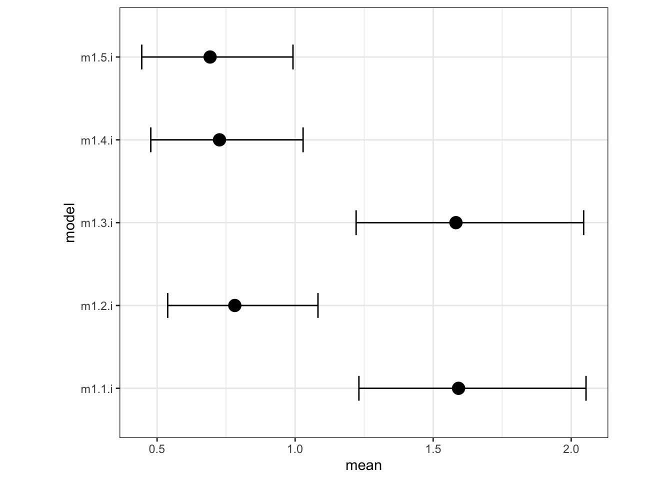
2. data(bangladesh) predicted proportions of women in each district using contraception, for both the fixed-effects model and the varying-effects model
In 1980, a typical Bengali woman could have 5 or more children in her lifetime. By the year 2000, a typical Bengali woman had only 2 or 3. You’re going to look at a historical set of data, when contraception was widely available but many families chose not to use it. These data reside in data(bangladesh) and come from the 1988 Bangladesh Fertility Survey. Each row is one of 1934 women. There are six variables, but you can focus on two of them for this practice problem:
(1) district: ID number of administrative district each woman resided in
(2) use.contraception: An indicator (0/1) of whether the woman was using contraception
Focus on predicting use.contraception, clustered by district_id. Fit both:
1) a traditional fixed-effects model that uses an index variable for district
2) a multilevel model with varying intercepts for district.
Plot the predicted proportions of women in each district using contraception, for both the fixed-effects model and the varying-effects model. That is, make a plot in which district ID is on the horizontal axis and expected proportion using contraception is on the vertical. Make one plot for each model, or layer them on the same plot, as you prefer. How do the models disagree? Can you explain the pattern of disagreement? In particular, can you explain the most extreme cases of disagreement, both why they happen where they do and why the models reach different inferences?**
library(rethinking)
data(bangladesh)
d <- bangladesh
The first thing to do is ensure that the cluster variable, district, is a contiguous set of integers. Recall that these values will be index values inside the model. If there are gaps, you’ll have parameters for which there is no data to inform them. Worse, the model probably won’t run. Look at the unique values of the district variable:
sort(unique(d$district))## [1] 1 2 3 4 5 6 7 8 9 10 11 12 13 14 15 16 17 18 19 20 21 22 23 24 25
## [26] 26 27 28 29 30 31 32 33 34 35 36 37 38 39 40 41 42 43 44 45 46 47 48 49 50
## [51] 51 52 53 55 56 57 58 59 60 61District 54 is absent. So district isn’t yet a good index variable, because it’s not contiguous. This is easy to fix. Just make a new variable that is contiguous. This is enough to do it:
d$district_id <- as.integer(as.factor(d$district))
sort(unique(d$district_id))
## [1] 1 2 3 4 5 6 7 8 9 10 11 12 13 14 15 16 17 18 19 20 21 22 23 24 25
## [26] 26 27 28 29 30 31 32 33 34 35 36 37 38 39 40 41 42 43 44 45 46 47 48 49 50
## [51] 51 52 53 54 55 56 57 58 59 60Now there are 60 values, contiguous integers 1 to 60.
2.1 traditional fixed-effects model that uses an index variable for district
2.1 rethinking
dat_list <- list(
C = d$use.contraception,
did = d$district_id
)

m2.1 <- ulam( alist(
C ~ bernoulli( p ),
logit(p) <- a[did],
a[did] ~ normal( 0 , 1.5 )
) , data=dat_list , chains=4 , cores=4 , log_lik=TRUE )

precis(m2.1, depth = 2)
## mean sd 5.5% 94.5% n_eff Rhat4
## a[1] -1.064615140 0.2082241 -1.40432883 -0.75001254 4061.973 0.9999862
## a[2] -0.581293145 0.4478574 -1.31131458 0.13142825 4634.026 0.9981715
## a[3] 1.238978258 1.2061872 -0.71925627 3.19793216 4621.404 0.9991591
## a[4] 0.008714590 0.3535837 -0.57192533 0.57051188 5342.413 0.9984687
## a[5] -0.570137783 0.3103432 -1.05275634 -0.08051717 4002.268 0.9992034
## a[6] -0.871427456 0.2676727 -1.30417055 -0.43914832 4735.133 0.9983993
## a[7] -0.887881645 0.4914059 -1.69169496 -0.11886997 4721.371 0.9988122
## a[8] -0.495628414 0.3389017 -1.03228605 0.03986791 5106.796 0.9990789
## a[9] -0.798449172 0.4254918 -1.50606516 -0.11693701 4652.507 0.9990507
## a[10] -1.960359811 0.7322881 -3.18977924 -0.84155010 4059.151 0.9990229
## a[11] -2.954270418 0.7908025 -4.30261004 -1.76821666 4490.882 0.9997145
## a[12] -0.607494145 0.3777830 -1.18192851 -0.01990514 4484.851 0.9984169
## a[13] -0.328839575 0.4027921 -0.98677717 0.30356849 3692.989 0.9990689
## a[14] 0.512178121 0.1851515 0.21564462 0.80406518 4930.125 1.0006198
## a[15] -0.535278129 0.4312011 -1.24416096 0.12718760 3568.023 0.9997864
## a[16] 0.189499628 0.4195215 -0.48670977 0.83774666 3734.701 0.9986811
## a[17] -0.846969403 0.4449759 -1.56625541 -0.16166096 3840.521 0.9985631
## a[18] -0.650087247 0.2928216 -1.12639702 -0.18848626 5901.460 0.9993198
## a[19] -0.456526548 0.3983769 -1.10630675 0.15878063 4277.559 0.9987468
## a[20] -0.372510883 0.4956593 -1.19585302 0.40251835 5641.624 0.9985031
## a[21] -0.413620070 0.4677454 -1.16162368 0.33121803 3823.727 0.9990337
## a[22] -1.286169288 0.5133405 -2.12372421 -0.51252059 3739.486 0.9994315
## a[23] -0.940094091 0.5629036 -1.86205513 -0.06887967 5201.407 0.9993709
## a[24] -2.026600274 0.7311232 -3.29087529 -0.92122375 3717.316 0.9989397
## a[25] -0.204810843 0.2325496 -0.56610041 0.16561313 4646.184 0.9989404
## a[26] -0.424639301 0.5467610 -1.32299396 0.46444436 4433.177 0.9982612
## a[27] -1.439012222 0.3685418 -2.06019482 -0.87807998 4266.607 0.9984892
## a[28] -1.102819022 0.3346034 -1.63572873 -0.58778877 5281.680 0.9982247
## a[29] -0.909835827 0.4021816 -1.55503776 -0.26835166 5434.367 0.9983089
## a[30] -0.036958166 0.2690816 -0.46409026 0.38251154 4950.974 0.9989412
## a[31] -0.181398991 0.3349239 -0.70968986 0.35421218 4911.337 0.9990865
## a[32] -1.264812879 0.4600333 -2.00425394 -0.54010357 3360.929 0.9990612
## a[33] -0.263230059 0.5260497 -1.14400586 0.54868790 5282.638 0.9984082
## a[34] 0.629116573 0.3590552 0.07184929 1.20582714 6076.060 0.9982203
## a[35] -0.008240447 0.2764201 -0.44729971 0.43002773 4764.968 0.9990490
## a[36] -0.588352020 0.4879081 -1.38687906 0.17725041 3523.430 0.9997752
## a[37] 0.140640293 0.5408706 -0.72203879 0.99973282 4471.215 0.9981874
## a[38] -0.848497573 0.5713210 -1.79587544 0.01438478 4226.401 0.9990882
## a[39] 0.010515960 0.3780320 -0.59715091 0.60163765 5647.856 0.9998906
## a[40] -0.137054470 0.3201771 -0.66263033 0.39435467 5593.324 0.9994658
## a[41] -0.002600673 0.3708684 -0.60181700 0.57193279 5943.443 0.9989207
## a[42] 0.162297163 0.5605841 -0.73657732 1.04128611 4465.620 0.9988026
## a[43] 0.128774664 0.2859080 -0.31021578 0.57822709 5607.019 0.9983842
## a[44] -1.191848050 0.4401132 -1.91336005 -0.50102954 3577.266 0.9992851
## a[45] -0.675717541 0.3413056 -1.23675668 -0.13881983 4532.647 0.9984789
## a[46] 0.091751865 0.2131878 -0.26235090 0.44546612 4172.205 0.9985585
## a[47] -0.126543465 0.5085578 -0.96117642 0.66138184 5456.306 0.9996449
## a[48] 0.100355900 0.3248770 -0.40355657 0.59861784 5537.638 0.9990882
## a[49] -1.730788841 1.0381395 -3.51132637 -0.14585214 5005.982 0.9989107
## a[50] -0.102996516 0.4408932 -0.80709414 0.60526787 4163.979 0.9989140
## a[51] -0.168095813 0.3323595 -0.70511145 0.36003011 5742.567 0.9992047
## a[52] -0.217835772 0.2624302 -0.63809146 0.20309194 5497.931 0.9983770
## a[53] -0.294696778 0.4472961 -1.00979141 0.41928815 4663.051 0.9994328
## a[54] -1.202080712 0.8365270 -2.57684737 0.08261446 4688.325 0.9982398
## a[55] 0.313583852 0.2940583 -0.15715332 0.78006066 3902.137 0.9990338
## a[56] -1.396734053 0.4634534 -2.13902116 -0.69130165 4191.758 0.9989519
## a[57] -0.172440186 0.3341429 -0.69156263 0.37256653 5530.796 0.9983794
## a[58] -1.724768458 0.7766282 -3.03392856 -0.60718512 3789.580 0.9997454
## a[59] -1.217470630 0.3965618 -1.86186638 -0.61011991 5459.312 0.9989427
## a[60] -1.255280757 0.3696653 -1.86012999 -0.67294274 6392.394 0.99863912.1 inla
library(brinla)
library(INLA)
library(tidyverse)

d2.i <- d %>%
  mutate(did= paste("d", as.integer(d$district_id), sep= "."),
         d.value= 1
         ) %>%
  spread(did, d.value)

#use this to quickly make a list of the index vbles to include in the model
did_formula <- paste("d", 1:60, sep=".", collapse = "+")


m2.1.i <- inla(use.contraception ~ d.1+d.2+d.3+d.4+d.5+d.6+d.7+d.8+d.9+d.10+d.11+d.12+d.13+d.14+d.15+d.16+d.17+d.18+d.19+d.20+d.21+d.22+d.23+d.24+d.25+d.26+d.27+d.28+d.29+d.30+d.31+d.32+d.33+d.34+d.35+d.36+d.37+d.38+d.39+d.40+d.41+d.42+d.43+d.44+d.45+d.46+d.47+d.48+d.49+d.50+d.51+d.52+d.53+d.54+d.55+d.56+d.57+d.58+d.59+d.60, data= d2.i, family = "binomial",
              Ntrials = 1, #Ntrials = 1 for bernoulli
              control.family = list(control.link=list(model="logit")),
              control.fixed = list(
        mean=  0 ,
        prec= 1/(1.5^2)),
              control.predictor=list(link=1, compute=T),
              control.compute=list(config=T, waic= TRUE))
summary(m2.1.i)
##
## Call:
## c("inla(formula = use.contraception ~ d.1 + d.2 + d.3 + d.4 + d.5 + ",
## " d.6 + d.7 + d.8 + d.9 + d.10 + d.11 + d.12 + d.13 + d.14 + ", " d.15
## + d.16 + d.17 + d.18 + d.19 + d.20 + d.21 + d.22 + d.23 + ", " d.24 +
## d.25 + d.26 + d.27 + d.28 + d.29 + d.30 + d.31 + d.32 + ", " d.33 +
## d.34 + d.35 + d.36 + d.37 + d.38 + d.39 + d.40 + d.41 + ", " d.42 +
## d.43 + d.44 + d.45 + d.46 + d.47 + d.48 + d.49 + d.50 + ", " d.51 +
## d.52 + d.53 + d.54 + d.55 + d.56 + d.57 + d.58 + d.59 + ", " d.60,
## family = \"binomial\", data = d2.i, Ntrials = 1, control.compute =
## list(config = T, ", " waic = TRUE), control.predictor = list(link = 1,
## compute = T), ", " control.family = list(control.link = list(model =
## \"logit\")), ", " control.fixed = list(mean = 0, prec = 1/(1.5^2)))")
## Time used:
## Pre = 5.32, Running = 0.54, Post = 0.847, Total = 6.71
## Fixed effects:
## mean sd 0.025quant 0.5quant 0.975quant mode kld
## (Intercept) -0.634 0.204 -1.035 -0.634 -0.234 -0.634 0
## d.1 -0.427 0.290 -1.001 -0.425 0.136 -0.421 0
## d.2 0.009 0.484 -0.967 0.017 0.936 0.034 0
## d.3 1.421 1.074 -0.583 1.382 3.640 1.306 0
## d.4 0.599 0.404 -0.194 0.600 1.391 0.600 0
## d.5 0.048 0.380 -0.709 0.052 0.782 0.060 0
## d.6 -0.247 0.333 -0.911 -0.244 0.397 -0.237 0
## d.7 -0.294 0.525 -1.367 -0.279 0.695 -0.250 0
## d.8 0.128 0.384 -0.636 0.131 0.871 0.138 0
## d.9 -0.183 0.471 -1.136 -0.173 0.713 -0.153 0
## d.10 -1.349 0.750 -2.950 -1.302 -0.002 -1.208 0
## d.11 -2.343 0.845 -4.166 -2.281 -0.851 -2.155 0
## d.12 -0.012 0.424 -0.861 -0.006 0.803 0.006 0
## d.13 0.274 0.443 -0.606 0.278 1.132 0.286 0
## d.14 1.138 0.276 0.599 1.137 1.681 1.136 0
## d.15 0.064 0.465 -0.869 0.071 0.957 0.085 0
## d.16 0.767 0.469 -0.148 0.766 1.692 0.762 0
## d.17 -0.239 0.467 -1.187 -0.229 0.649 -0.208 0
## d.18 -0.030 0.360 -0.747 -0.027 0.666 -0.019 0
## d.19 0.150 0.434 -0.716 0.155 0.987 0.165 0
## d.20 0.200 0.530 -0.863 0.208 1.220 0.223 0
## d.21 0.161 0.497 -0.834 0.168 1.117 0.182 0
## d.22 -0.673 0.542 -1.796 -0.652 0.332 -0.611 0
## d.23 -0.337 0.566 -1.501 -0.318 0.724 -0.282 0
## d.24 -1.413 0.743 -3.001 -1.367 -0.079 -1.272 0
## d.25 0.413 0.314 -0.205 0.413 1.027 0.415 0
## d.26 0.139 0.563 -0.994 0.149 1.216 0.169 0
## d.27 -0.826 0.418 -1.679 -0.814 -0.037 -0.791 0
## d.28 -0.476 0.377 -1.235 -0.470 0.244 -0.456 0
## d.29 -0.291 0.424 -1.148 -0.283 0.517 -0.266 0
## d.30 0.585 0.321 -0.046 0.585 1.214 0.585 0
## d.31 0.428 0.392 -0.347 0.429 1.193 0.432 0
## d.32 -0.641 0.502 -1.676 -0.624 0.296 -0.590 0
## d.33 0.304 0.541 -0.775 0.310 1.348 0.322 0
## d.34 1.222 0.394 0.461 1.217 2.008 1.208 0
## d.35 0.612 0.345 -0.066 0.612 1.289 0.612 0
## d.36 0.020 0.514 -1.018 0.030 1.002 0.049 0
## d.37 0.693 0.551 -0.384 0.692 1.777 0.690 0
## d.38 -0.252 0.574 -1.428 -0.235 0.825 -0.200 0
## d.39 0.594 0.425 -0.241 0.595 1.427 0.595 0
## d.40 0.467 0.364 -0.251 0.468 1.178 0.470 0
## d.41 0.594 0.425 -0.241 0.595 1.427 0.595 0
## d.42 0.703 0.587 -0.445 0.701 1.859 0.698 0
## d.43 0.739 0.353 0.048 0.739 1.433 0.737 0
## d.44 -0.575 0.474 -1.546 -0.561 0.316 -0.532 0
## d.45 -0.061 0.384 -0.828 -0.056 0.680 -0.047 0
## d.46 0.713 0.293 0.139 0.713 1.288 0.712 0
## d.47 0.447 0.523 -0.590 0.450 1.464 0.456 0
## d.48 0.700 0.360 -0.006 0.700 1.408 0.699 0
## d.49 -1.230 1.047 -3.465 -1.166 0.651 -1.035 0
## d.50 0.483 0.478 -0.461 0.485 1.415 0.489 0
## d.51 0.449 0.377 -0.294 0.451 1.185 0.453 0
## d.52 0.391 0.323 -0.244 0.392 1.022 0.394 0
## d.53 0.286 0.482 -0.675 0.290 1.219 0.300 0
## d.54 -0.669 0.837 -2.437 -0.625 0.856 -0.537 0
## d.55 0.913 0.355 0.221 0.912 1.613 0.909 0
## d.56 -0.777 0.495 -1.799 -0.759 0.144 -0.724 0
## d.57 0.428 0.392 -0.347 0.429 1.193 0.432 0
## d.58 -1.120 0.776 -2.772 -1.074 0.278 -0.980 0
## d.59 -0.601 0.448 -1.514 -0.588 0.243 -0.563 0
## d.60 -0.635 0.409 -1.465 -0.625 0.140 -0.606 0
##
## Expected number of effective parameters(stdev): 54.05(0.00)
## Number of equivalent replicates : 35.78
##
## Watanabe-Akaike information criterion (WAIC) ...: 2521.28
## Effective number of parameters .................: 52.54
##
## Marginal log-Likelihood: -1291.66
## Posterior marginals for the linear predictor and
## the fitted values are computed2.2 varying intercepts model
2.2 rethinking
m2.2 <- ulam( alist(
C ~ bernoulli( p ),
logit(p) <- a[did],
a[did] ~ normal( a_bar , sigma ),
a_bar ~ normal( 0 , 1.5 ),
sigma ~ exponential( 1 )
) ,data=dat_list , chains=4 , cores=4 , log_lik=TRUE )

precis(m2.2, depth= 2)
## mean sd 5.5% 94.5% n_eff Rhat4
## a[1] -0.993304390 0.19685939 -1.30352873 -0.678219180 4017.788 0.9993184
## a[2] -0.597595188 0.35714055 -1.18357290 -0.049149635 3610.315 0.9981816
## a[3] -0.225976383 0.52450600 -1.03896674 0.646063974 2709.746 1.0014249
## a[4] -0.182389563 0.30613876 -0.65606104 0.307375975 3137.912 0.9989681
## a[5] -0.573478048 0.28819658 -1.02926294 -0.111002250 3833.507 0.9987476
## a[6] -0.811512433 0.24116536 -1.20032312 -0.433749476 2776.128 0.9990751
## a[7] -0.758406236 0.36360947 -1.35702669 -0.201105775 2715.380 1.0009859
## a[8] -0.515030875 0.28882052 -0.96410438 -0.058353283 4045.075 0.9989817
## a[9] -0.702757894 0.33405359 -1.22684793 -0.177234470 4092.655 0.9981603
## a[10] -1.140229991 0.44080539 -1.87250117 -0.481014664 2558.113 0.9988190
## a[11] -1.546932076 0.43832884 -2.27304504 -0.876803144 1978.861 1.0004264
## a[12] -0.597558560 0.30609300 -1.10299471 -0.120462986 4023.984 0.9991525
## a[13] -0.417077352 0.32543435 -0.94363754 0.090991813 2945.958 0.9995410
## a[14] 0.389478787 0.18663821 0.09458163 0.678357215 3713.085 0.9999555
## a[15] -0.560099999 0.34265111 -1.09543297 -0.026923050 3856.655 0.9992835
## a[16] -0.121972607 0.34673869 -0.67295516 0.432792182 3992.755 0.9992727
## a[17] -0.736254270 0.34914749 -1.30344587 -0.192370376 3287.564 0.9985646
## a[18] -0.634505418 0.25281541 -1.02872620 -0.251900095 3955.191 0.9990841
## a[19] -0.510359242 0.33501628 -1.05484210 0.010862623 3200.847 0.9985103
## a[20] -0.487107364 0.38369446 -1.11211091 0.133133054 3510.082 1.0010417
## a[21] -0.495112115 0.34919931 -1.04780684 0.051488044 2623.920 0.9989965
## a[22] -0.964029737 0.36076223 -1.54951006 -0.410145093 3237.638 1.0003007
## a[23] -0.764828381 0.40012196 -1.40523717 -0.143959596 3261.625 0.9995192
## a[24] -1.173536876 0.43015615 -1.88710746 -0.529348570 2243.143 1.0016510
## a[25] -0.281136009 0.22840422 -0.65060411 0.080329145 3640.760 1.0005751
## a[26] -0.515704168 0.38397574 -1.12648638 0.075543740 4105.619 0.9988569
## a[27] -1.182153513 0.31096705 -1.69038066 -0.705540317 2327.422 0.9983693
## a[28] -0.961938053 0.27750475 -1.41623742 -0.535994123 3099.290 0.9988519
## a[29] -0.800449652 0.32076170 -1.34375160 -0.279396778 2610.240 0.9997740
## a[30] -0.128150323 0.24848960 -0.52182993 0.258486913 4077.103 1.0002312
## a[31] -0.293927220 0.29649430 -0.78176738 0.172880733 3981.867 0.9985721
## a[32] -0.971057693 0.35480068 -1.55674523 -0.443598662 2843.469 0.9988210
## a[33] -0.425368437 0.38487659 -1.03396344 0.208808398 3369.482 0.9984469
## a[34] 0.275093725 0.29786165 -0.18572351 0.770223132 2921.080 0.9995001
## a[35] -0.132698116 0.24732778 -0.53222052 0.272571045 3878.541 0.9993393
## a[36] -0.577593237 0.36733515 -1.18273084 0.005909177 2941.705 0.9987964
## a[37] -0.228401045 0.39581613 -0.84583721 0.415666450 3621.821 0.9989829
## a[38] -0.714860908 0.38692198 -1.33906518 -0.111934187 3374.444 0.9996506
## a[39] -0.210459939 0.31610647 -0.71008984 0.307614885 3673.804 0.9989087
## a[40] -0.259044721 0.26648465 -0.68198684 0.173031176 3800.753 0.9991202
## a[41] -0.199786547 0.32143292 -0.71962544 0.307810713 3311.606 0.9992730
## a[42] -0.240093832 0.39633001 -0.85430021 0.397062768 3511.029 0.9980482
## a[43] -0.040698814 0.25714973 -0.45686841 0.377982369 3994.844 0.9986478
## a[44] -0.957262737 0.33641348 -1.47872663 -0.433582252 3713.045 0.9988768
## a[45] -0.654602802 0.28287621 -1.12409480 -0.199625111 3254.606 0.9982511
## a[46] -0.007606195 0.20017458 -0.32812219 0.318976523 3776.049 0.9991054
## a[47] -0.345680976 0.37437161 -0.95472098 0.231408734 2883.513 0.9990565
## a[48] -0.079558299 0.26749072 -0.50859177 0.353508636 4105.345 0.9993870
## a[49] -0.861924273 0.46774277 -1.61462553 -0.125447854 2948.914 0.9984541
## a[50] -0.303562746 0.35179952 -0.86211052 0.264697399 4083.645 0.9991216
## a[51] -0.274355622 0.28377285 -0.72463306 0.173123338 3594.329 0.9992729
## a[52] -0.304527845 0.23581559 -0.67864921 0.086637326 3068.919 0.9992677
## a[53] -0.424290123 0.34537637 -0.98584725 0.132592438 3532.797 0.9997970
## a[54] -0.786308464 0.43439768 -1.47568587 -0.094263529 3183.325 0.9990603
## a[55] 0.094144686 0.25510453 -0.30923387 0.518123164 3422.667 1.0000150
## a[56] -1.071383597 0.36334328 -1.66748994 -0.517147253 2852.532 0.9992121
## a[57] -0.299766961 0.31037823 -0.80212431 0.188303467 3192.180 0.9990816
## a[58] -0.999199065 0.42703203 -1.70643843 -0.337866028 3249.540 0.9997235
## a[59] -0.997996081 0.31096154 -1.50901261 -0.521482943 2676.881 0.9991911
## a[60] -1.054032303 0.29581217 -1.52894761 -0.591752017 3288.263 0.9988056
## a_bar -0.538938409 0.08556773 -0.67563777 -0.403003761 1671.004 1.0000150
## sigma 0.517696556 0.08155719 0.39484305 0.653368298 710.658 1.00145792.2 inla
m2.2.i <- inla(use.contraception ~ f(district_id, model="iid"), data= d2.i, family = "binomial",
              Ntrials = 1, #Ntrials = 1 for bernoulli
              control.family = list(control.link=list(model="logit")),
              control.fixed = list(
        mean.intercept=  0 ,
        prec.intercept= 1/(1.5^2)),
              control.predictor=list(link=1, compute=T),
              control.compute=list(config=T, waic= TRUE))
summary(m2.2.i)
##
## Call:
## c("inla(formula = use.contraception ~ f(district_id, model = \"iid\"),
## ", " family = \"binomial\", data = d2.i, Ntrials = 1, control.compute =
## list(config = T, ", " waic = TRUE), control.predictor = list(link = 1,
## compute = T), ", " control.family = list(control.link = list(model =
## \"logit\")), ", " control.fixed = list(mean.intercept = 0,
## prec.intercept = 1/(1.5^2)))" )
## Time used:
## Pre = 1.39, Running = 1.09, Post = 0.24, Total = 2.72
## Fixed effects:
## mean sd 0.025quant 0.5quant 0.975quant mode kld
## (Intercept) -0.532 0.084 -0.701 -0.531 -0.371 -0.528 0
##
## Random effects:
## Name Model
## district_id IID model
##
## Model hyperparameters:
## mean sd 0.025quant 0.5quant 0.975quant mode
## Precision for district_id 4.72 1.64 2.38 4.43 8.72 3.95
##
## Expected number of effective parameters(stdev): 33.99(4.22)
## Number of equivalent replicates : 56.89
##
## Watanabe-Akaike information criterion (WAIC) ...: 2514.73
## Effective number of parameters .................: 33.32
##
## Marginal log-Likelihood: -1278.85
## Posterior marginals for the linear predictor and
## the fitted values are computedbri.hyperpar.summary(m2.2.i)## mean sd q0.025 q0.5 q0.975 mode
## SD for district_id 0.4799258 0.07896337 0.3386648 0.4748904 0.6490116 0.4657571Side note: this is how you calculate the sd from the hyperprior (\(\sigma\))
bri.hyperpar.summary(m2.2.i)## mean sd q0.025 q0.5 q0.975 mode
## SD for district_id 0.4799258 0.07896337 0.3386648 0.4748904 0.6490116 0.4657571# hyperparameter of the precision
m2.2.i.prec <- m2.2.i$internal.marginals.hyperpar
#transform precision to sd using inla.tmarginal
#m2.2.i.prec[[1]] is used to access the actual values inside the list
m2.2.i.sd <- inla.tmarginal(function(x) sqrt(exp(-x)), m2.2.i.prec[[1]])
#plot the post of the sd per district (sigma)
plot(m2.2.i.sd)
#summary stats for the sd
m2.2.i.sd.sum <- inla.zmarginal(m2.2.i.sd)
## Mean 0.479926
## Stdev 0.0789634
## Quantile 0.025 0.338665
## Quantile 0.25 0.424458
## Quantile 0.5 0.47489
## Quantile 0.75 0.529788
## Quantile 0.975 0.649012# this coincides perfectly with the result from bri.hyperpar.summary2.3 plot of posterior mean probabilities in each district
Now let’s extract the samples, compute posterior mean probabilities in each district, and plot it all:
plot rethinking
post1 <- extract.samples( m2.1 )
post2 <- extract.samples( m2.2 )
p1 <- apply( inv_logit(post1$a) , 2 , mean )
p2 <- apply( inv_logit(post2$a) , 2 , mean )
nd <- max(dat_list$did)
plot( NULL , xlim=c(1,nd) , ylim=c(0,1) , ylab="prob use contraception" , xlab="district" )
points( 1:nd , p1 , pch=16 , col=rangi2 )
points( 1:nd , p2 )
abline( h=mean(inv_logit(post2$a_bar)) , lty=2 )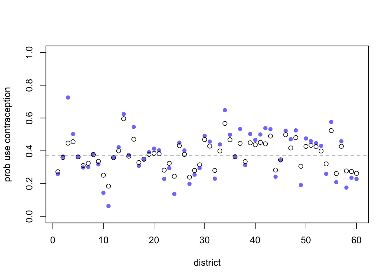
plot inla
https://people.bath.ac.uk/jjf23/inla/oneway.html
https://people.bath.ac.uk/jjf23/brinla/reeds.html
posterior mean for each district a for the idex fixed effect model m2.1:
# m2.2.i$summary.fixed[[1]] would gives us the summary we want but not in the response scale, we need to  transform it using the inverse logit

inverse_logit <- function (x){
    p <- 1/(1 + exp(-x))
    p <- ifelse(x == Inf, 1, p)
    p }

#inla.tmarginal : apply inverse logit to all district marginals
#inla.zmarginal : summary of the logit-transformed marginals
# we eliminate the first element of this list, the intercept.
m2.1.i.fix<- lapply(m2.1.i$marginals.fixed, function (x) inla.zmarginal( inla.tmarginal (inverse_logit, x )))[-1]
posterior mean for each district a for the varying intercept model m2.2:
# m2.2.i$summary.random[[1]] would gives us the summary we want but not in the response scale, we need to  transform it using the inverse logit

#inla.tmarginal : apply inverse logit to all district marginals
#inla.zmarginal : summary of the logit-transformed marginals
m2.2.i.rand<- lapply(m2.2.i$marginals.random$district_id, function (x) inla.zmarginal( inla.tmarginal (inverse_logit, x )))
# sapply(m2.2.i.rand, function(x) x[1]) extracts the first element (the mean) from the summary of the posterior of each district
m2.i.mean <- bind_cols(district= 1:60,mean.m2.1= unlist(sapply(m2.1.i.fix, function(x) x[1])), mean.m2.2=unlist(sapply(m2.2.i.rand, function(x) x[1])))
m2.2.i.abar <- inla.zmarginal( inla.tmarginal (inverse_logit, m2.2.i$marginals.fixed[["(Intercept)"]] ))## Mean 0.370149
## Stdev 0.0193718
## Quantile 0.025 0.331663
## Quantile 0.25 0.357164
## Quantile 0.5 0.37022
## Quantile 0.75 0.383175
## Quantile 0.975 0.407995m2.i.district.plot <- ggplot() +
geom_point(data= m2.i.mean, aes(x= district, y= mean.m2.1), color= "blue", alpha= 0.5)+
geom_point(data= m2.i.mean, aes(x= district, y= mean.m2.2), color= "black", alpha= 0.5, shape= 1)+
geom_hline(yintercept=m2.2.i.abar[[1]], linetype='longdash') +
ylim(0,1)+
labs(y = "prob use contraception")+
theme_bw()
m2.i.district.plot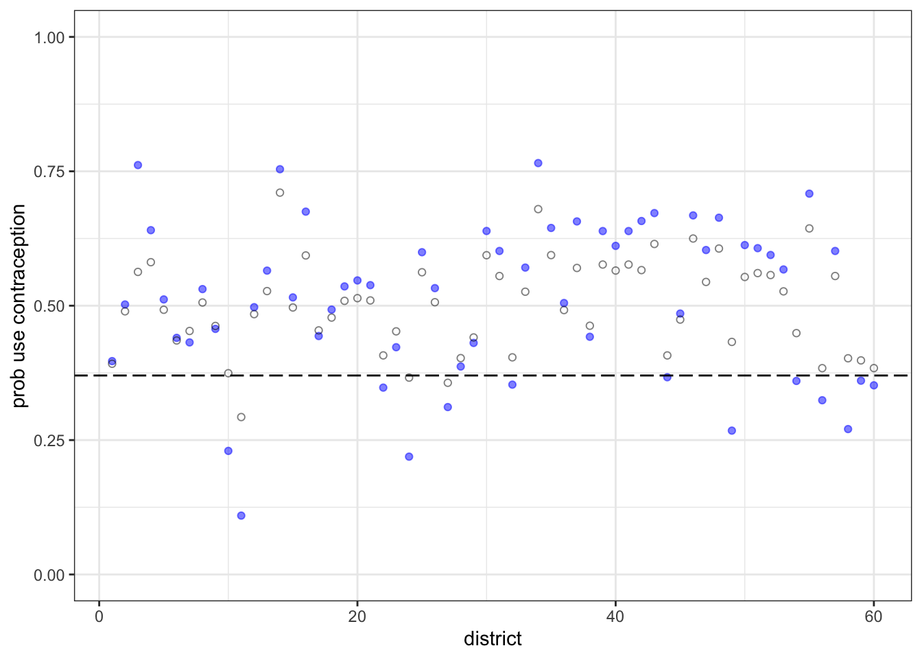
The blue points are the fixed estimations. The open points are the varying effects. As you’d expect, they are shrunk towards the mean (the dashed line). Some are shrunk more than others. The third district from the left shrunk a lot.
Let’s look at the sample size in each district:
table(d$district_id)##
## 1 2 3 4 5 6 7 8 9 10 11 12 13 14 15 16 17 18 19 20
## 117 20 2 30 39 65 18 37 23 13 21 29 24 118 22 20 24 47 26 15
## 21 22 23 24 25 26 27 28 29 30 31 32 33 34 35 36 37 38 39 40
## 18 20 15 14 67 13 44 49 32 61 33 24 14 35 48 17 13 14 26 41
## 41 42 43 44 45 46 47 48 49 50 51 52 53 54 55 56 57 58 59 60
## 26 11 45 27 39 86 15 42 4 19 37 61 19 6 45 27 33 10 32 42District 3 has only 2 women sampled. So it shrinks a lot. There are couple of other districts, like 49 and 54, that also have very few women sampled. But their fixed estimates aren’t as extreme, so they don’t shrink as much as district 3 does. All of this is explained by partial pooling, of course.