Statistical Rethinking 2nd edition Homework 5 in INLA
library(tidyverse)
library(rethinking)
library(dagitty)
library(INLA)
library(knitr)
library(stringr)
1. data(Wines2012) consider only variation among judges and wines
Consider the data (Wines2012) data table.These data are expert ratings of 20 different French and American wines by 9 different French and American judges. Your goal is to model score, the subjective rating assigned by each judge to each wine. I recommend standardizing it.
In this first problem, consider only variation among judges and wines. Construct index variables of judge and wine and then use these index variables to construct a linear regression model. Justify your priors. You should end up with 9 judge parameters and 20 wine parameters. Use ulam instead of quap to build this model, and be sure to check the chains for convergence. If you’d rather build the model directly in Stan or PyMC3, go ahead. I just want you to use Hamiltonian Monte Carlo instead of quadratic approximation. How do you interpret the variation among individual judges and individual wines? Do you notice any patterns, just by plotting the differences? Which judges gave the highest/lowest ratings? Which wines were rated worst/ best on average?
library(rethinking)
data(Wines2012)
d <- Wines2012

dat_list <- list(
    S = standardize(d$score),
    jid = as.integer(d$judge),
    wid = as.integer(d$wine)
)

str(dat_list)
## List of 3
## $ S : num [1:180] -1.5766 -0.4505 -0.0751 0.3003 -2.3274 ...
## ..- attr(*, "scaled:center")= num 14.2
## ..- attr(*, "scaled:scale")= num 2.66
## $ jid: int [1:180] 4 4 4 4 4 4 4 4 4 4 ...
## $ wid: int [1:180] 1 3 5 7 9 11 13 15 17 19 ...The model is straightforward. The only issue is the priors. Since I’ve standardized the outcome, we can use the ordinary N(0,0.5) prior from the examples in the text with standardized outcomes. Then the prior outcomes will stay largely within the possible outcome space. A bit more regularization than that wouldn’t be a bad idea either.
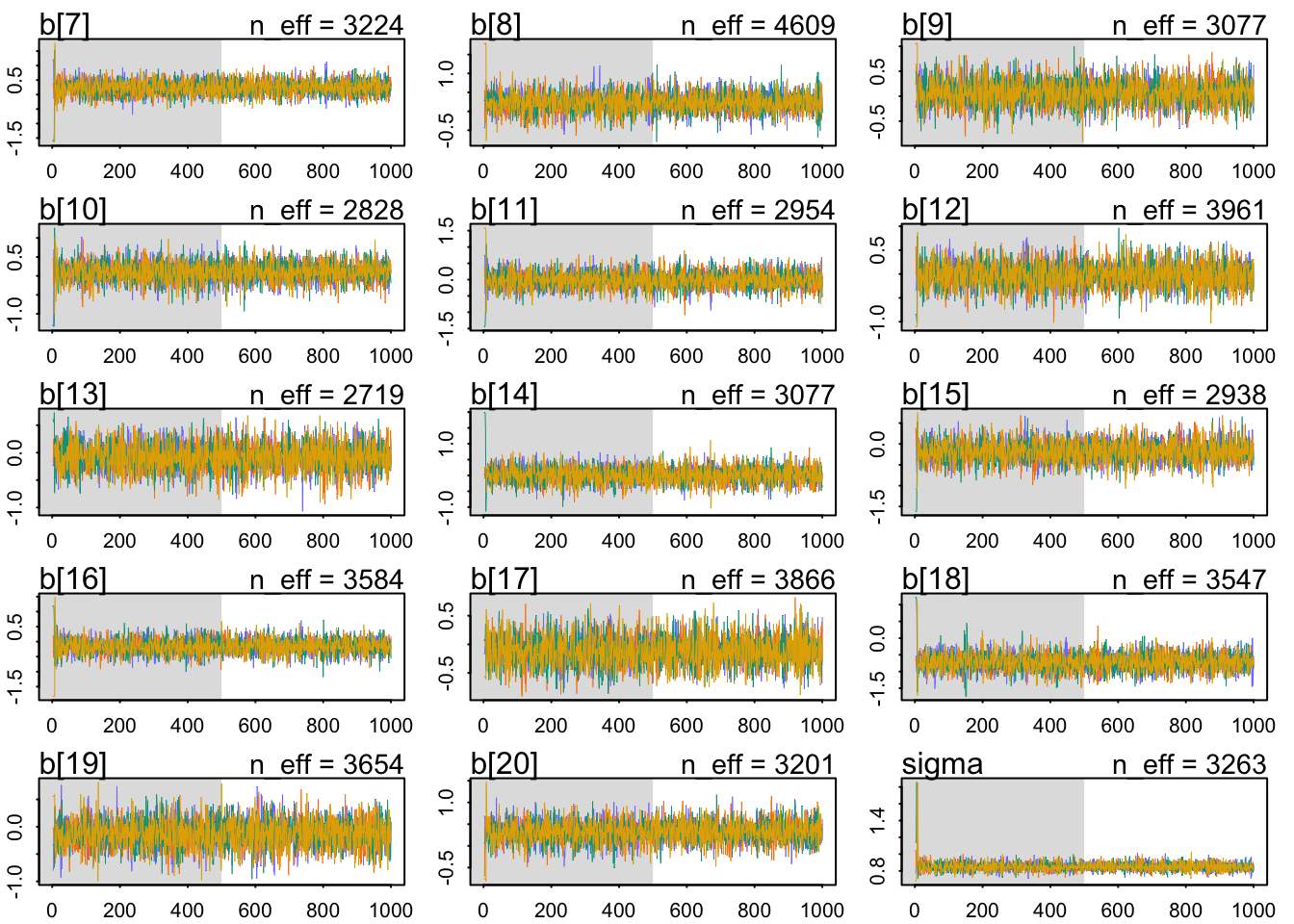
diagnostics that precis provides: The n_eff values are all actually higher than the number of samples (2000), and all the Rhat values at exactly 1. Looks good so far. These diagnostics can mislead, however, so let’s look at the trace plots too: These pass the hairy-caterpillar-ocular-inspection-test: all the chains mix in the same region, and they move quickly through it, not getting stuck anyplace. Now let’s plot these parameters so they are easier to interpret:
1. rethinking
#How do you interpret the variation among individual judges and individual wines?
#Do you notice any patterns, just by plotting the differences? Which judges gave the highest/lowest ratings? Which wines were rated worst/ best on average?

m1 <- ulam(
  alist(
    S ~ dnorm(mu, sigma),
    mu <- a[jid] + b[wid],
    a[jid] ~ dnorm(0, 0.5),
    b[wid] ~ dnorm(0, 0.5),
    sigma ~dexp(1)

  ), data=dat_list, chains=4 , cores=4)

precis(m1, 2)
## mean sd 5.5% 94.5% n_eff Rhat4
## a[1] -0.28456935 0.18244849 -0.57655372 0.007940745 2337.546 0.9987276
## a[2] 0.20620935 0.19891832 -0.10529185 0.526439589 2401.703 0.9986654
## a[3] 0.20104814 0.19327657 -0.10378734 0.515449300 2507.671 0.9991754
## a[4] -0.54908667 0.18545137 -0.84727888 -0.250156595 2054.116 0.9995357
## a[5] 0.78312014 0.18924306 0.47471264 1.083629540 2066.952 0.9987144
## a[6] 0.46468818 0.19656102 0.14122244 0.774990187 2868.345 0.9987185
## a[7] 0.12534703 0.19358745 -0.19112406 0.431617002 2122.989 0.9989241
## a[8] -0.65681781 0.19765859 -0.97138649 -0.347380359 2423.641 0.9984746
## a[9] -0.35382508 0.19091203 -0.64930455 -0.046985129 2468.202 0.9990944
## b[1] 0.12576225 0.25245369 -0.27622219 0.532855185 3189.370 0.9989837
## b[2] 0.09487463 0.25305174 -0.30059851 0.493873764 3380.437 0.9983242
## b[3] 0.23394061 0.25843820 -0.18948039 0.643586921 3084.082 0.9986572
## b[4] 0.47516853 0.25360756 0.06494031 0.880570578 2759.755 0.9987220
## b[5] -0.10018953 0.26904416 -0.51848074 0.341992520 3603.007 0.9993904
## b[6] -0.30511432 0.25722615 -0.71453007 0.107363031 3243.426 0.9988293
## b[7] 0.25013892 0.25579423 -0.17192054 0.652582797 3224.042 0.9983954
## b[8] 0.23482461 0.25523562 -0.16579080 0.656578423 4608.826 0.9985614
## b[9] 0.07743381 0.24942789 -0.32651375 0.472886967 3076.735 0.9986942
## b[10] 0.11065175 0.26301421 -0.32687385 0.523688968 2828.181 0.9989681
## b[11] -0.01253733 0.26748273 -0.41489668 0.423804175 2953.959 0.9995380
## b[12] -0.01561847 0.26136100 -0.43208123 0.402551769 3961.068 0.9982981
## b[13] -0.08633619 0.25624363 -0.49212819 0.327378630 2718.963 0.9986956
## b[14] 0.02049832 0.26755859 -0.41973850 0.450164176 3077.406 0.9987507
## b[15] -0.17537163 0.25870130 -0.58214874 0.243659740 2938.236 0.9987985
## b[16] -0.15715860 0.25612563 -0.56939030 0.248434740 3584.190 0.9986760
## b[17] -0.11108560 0.25548478 -0.53921987 0.296133255 3866.343 0.9985989
## b[18] -0.71224101 0.26681182 -1.14505477 -0.286406405 3546.807 0.9984760
## b[19] -0.12961389 0.26213113 -0.54021521 0.288183086 3654.057 0.9988095
## b[20] 0.32867082 0.25098577 -0.06766971 0.734961386 3201.377 0.9991989
## sigma 0.84743607 0.04697524 0.77516782 0.928286153 3262.519 0.9999055traceplot(m1)## [1] 1000
## [1] 1
## [1] 1000## Waiting to draw page 2 of 2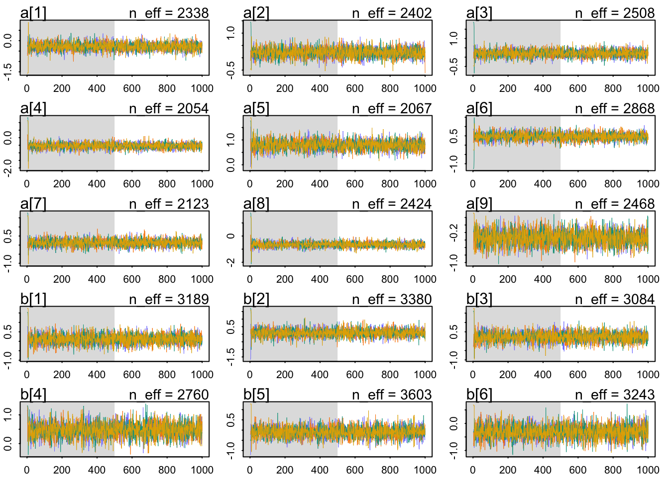
plot(precis(m1, 2))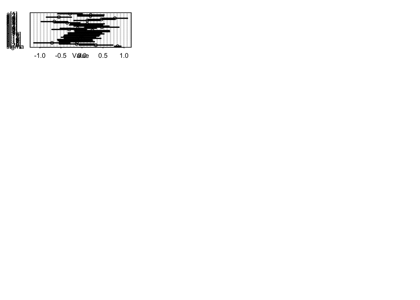
1. INLA
In order to code a separate intercept for each judge and wine, we need to reformat the data so that there are separate variables for each intercept, with 1s for a given value of the variable we are basing the intercept on and NAs for all other values.
d.i <- d %>%
  mutate(S = standardize(d$score),
    jid = paste("j",as.integer(d$judge), sep= "."),
    wid =  paste("w",as.integer(d$wine), sep= "."),
    j.value= 1,
    w.value= 1) %>%
  spread(jid, j.value) %>%
  spread(wid, w.value)

j <- paste("j", 1:9, sep=".")

w <- paste("w", 1:20, sep=".")

est <- c(j,w)

m1.i<- inla(S~ -1 +j.1+ j.2+j.3+j.4+j.5+j.6+j.7+j.8+j.9+
                          w.1+w.2+ w.3+w.4+w.5+w.6+w.7+w.8+w.9+w.10+w.11+w.12+w.13+w.14+w.15+ w.16+w.17+ w.18+w.19+w.20, data= d.i,
                        control.fixed = list(
        mean= 0,
        prec= 0.5),
        control.compute = list(dic=TRUE, waic= TRUE)
)

summary(m1.i )
##
## Call:
## c("inla(formula = S ~ -1 + j.1 + j.2 + j.3 + j.4 + j.5 + j.6 + j.7 + ",
## " j.8 + j.9 + w.1 + w.2 + w.3 + w.4 + w.5 + w.6 + w.7 + w.8 + ", " w.9
## + w.10 + w.11 + w.12 + w.13 + w.14 + w.15 + w.16 + w.17 + ", " w.18 +
## w.19 + w.20, data = d.i, control.compute = list(dic = TRUE, ", " waic =
## TRUE), control.fixed = list(mean = 0, prec = 0.5))" )
## Time used:
## Pre = 3.18, Running = 0.284, Post = 0.44, Total = 3.9
## Fixed effects:
## mean sd 0.025quant 0.5quant 0.975quant mode kld
## j.1 -0.313 0.320 -0.941 -0.313 0.314 -0.313 0
## j.2 0.240 0.320 -0.388 0.240 0.867 0.240 0
## j.3 0.230 0.320 -0.397 0.230 0.858 0.230 0
## j.4 -0.608 0.320 -1.236 -0.608 0.019 -0.608 0
## j.5 0.894 0.320 0.266 0.894 1.522 0.894 0
## j.6 0.535 0.320 -0.093 0.535 1.162 0.535 0
## j.7 0.147 0.320 -0.480 0.147 0.775 0.148 0
## j.8 -0.737 0.320 -1.365 -0.738 -0.110 -0.738 0
## j.9 -0.387 0.320 -1.015 -0.387 0.240 -0.387 0
## w.1 0.148 0.377 -0.593 0.148 0.889 0.148 0
## w.2 0.108 0.377 -0.633 0.108 0.849 0.108 0
## w.3 0.289 0.377 -0.452 0.289 1.029 0.289 0
## w.4 0.590 0.377 -0.152 0.590 1.330 0.590 0
## w.5 -0.132 0.377 -0.873 -0.132 0.608 -0.132 0
## w.6 -0.393 0.377 -1.134 -0.393 0.348 -0.393 0
## w.7 0.309 0.377 -0.432 0.309 1.049 0.309 0
## w.8 0.289 0.377 -0.452 0.289 1.029 0.289 0
## w.9 0.088 0.377 -0.653 0.088 0.829 0.088 0
## w.10 0.128 0.377 -0.613 0.128 0.869 0.128 0
## w.11 -0.012 0.377 -0.753 -0.012 0.728 -0.012 0
## w.12 -0.032 0.377 -0.773 -0.032 0.708 -0.032 0
## w.13 -0.112 0.377 -0.853 -0.112 0.628 -0.112 0
## w.14 0.008 0.377 -0.733 0.008 0.748 0.008 0
## w.15 -0.233 0.377 -0.974 -0.233 0.508 -0.233 0
## w.16 -0.213 0.377 -0.954 -0.213 0.528 -0.213 0
## w.17 -0.152 0.377 -0.893 -0.152 0.588 -0.152 0
## w.18 -0.914 0.377 -1.655 -0.915 -0.174 -0.915 0
## w.19 -0.172 0.377 -0.913 -0.172 0.568 -0.173 0
## w.20 0.409 0.377 -0.332 0.409 1.149 0.409 0
##
## Model hyperparameters:
## mean sd 0.025quant 0.5quant
## Precision for the Gaussian observations 1.41 0.159 1.11 1.40
## 0.975quant mode
## Precision for the Gaussian observations 1.74 1.39
##
## Expected number of effective parameters(stdev): 27.12(0.101)
## Number of equivalent replicates : 6.64
##
## Deviance Information Criterion (DIC) ...............: 481.08
## Deviance Information Criterion (DIC, saturated) ....: 211.59
## Effective number of parameters .....................: 28.36
##
## Watanabe-Akaike information criterion (WAIC) ...: 482.39
## Effective number of parameters .................: 26.24
##
## Marginal log-Likelihood: -273.56
## Posterior marginals for the linear predictor and
## the fitted values are computed## Pull out summaries from the model object
m1.i.sum <- summary(m1.i)
## Summarise results
m1.i.df <- data.frame(mean = m1.i.sum$fixed[,"mean"],
lower = m1.i.sum$fixed[,"0.025quant"],
upper = m1.i.sum$fixed[,"0.975quant"],
stringsAsFactors = FALSE)
mi.i.df <- bind_cols(as.factor(est), m1.i.df)## New names:
## * NA -> ...1m1.i.plot <- mi.i.df %>%
mutate(est= factor(est, levels= c("j.1", "j.2" , "j.3" , "j.4" , "j.5" ,"j.6" , "j.7" , "j.8" , "j.9" , "w.1" , "w.2" , "w.3" , "w.4" , "w.5" , "w.6" , "w.7" ,"w.8" , "w.9" ,"w.10" ,"w.11", "w.12" ,"w.13" ,"w.14", "w.15" ,"w.16", "w.17", "w.18", "w.19", "w.20"))) %>%
ggplot() +
geom_pointrange(aes(x = factor(est), y = mean, ymin = lower, ymax = upper), position = position_dodge(0.5)) +
xlab("coefficient") +
ylab("Estimate")+
coord_flip()+
theme_bw()
m1.i.plot 
The a/j parameters are the judges. Each represents an average deviation of the scores. So judges with lower values are harsher on average. Judges with higher values liked the wines more on average. There is some noticeable variation here. It is fairly easy to tell the judges apart.
The w parameters are the wines. Each represents an average score across all judges. Except for wine 18 (a New Jersey red I think), there isn’t that much variation. These are good wines, after all. Overall, there is more variation from judge than from wine.
2. data(Wines2012) consider three features of the wines and judges: flight, wine.amer, judge.amer
Now consider three features of the wines and judges:
flight: Whether the wine is red or white.
wine.amer: Indicator variable for American wines.
judge.amer: Indicator variable for American judges.
Use indicator or index variables to model the influence of these features on the scores. Omit the individual judge and wine index variables from Problem 1. Do not include interaction effects yet. Again use ulam, justify your priors, and be sure to check the chains. What do you conclude about the differences among the wines and judges? Try to relate the results to the inferences in Problem 1.
The easiest way to code the data is to use indicator variables. Let’s look at that approach first. I’ll do an index variable version next. I’ll use the three indicator variables W (NJ wine), J (American NJ), and R (red wine).
2.a indicator variables
2.a rethinking
dat_list2 <- list(
    S = standardize(d$score),
    W = d$wine.amer,
    J = d$judge.amer,
    F= if_else(d$flight == "white", 0, 1))

m2a <- ulam(
  alist(
    S ~ dnorm(mu, sigma),
    mu <- a + bW*W + bJ*J + bF*F,
    a ~ dnorm(0, 0.2),
    bW~ dnorm(0, 0.5),
    bJ~ dnorm(0, 0.5),
    bF~ dnorm(0, 0.5),
  sigma ~ dexp(1)
    ), data=dat_list2, chains=4 , cores=4)

precis(m2a)
## mean sd 5.5% 94.5% n_eff Rhat4
## a -0.015106047 0.12659361 -0.2150224636 0.1881938 1595.729 1.0011814
## bW -0.180550118 0.13893182 -0.4002781036 0.0489065 1756.814 0.9987974
## bJ 0.225884935 0.14068947 -0.0001966947 0.4466232 1728.246 1.0001453
## bF -0.004929157 0.13457742 -0.2262693044 0.2063808 1738.007 1.0001428
## sigma 0.999968848 0.05261749 0.9225525370 1.0880751 1828.629 0.9987323traceplot(m2a)## [1] 1000
## [1] 1
## [1] 1000plot(precis(m2a, 2))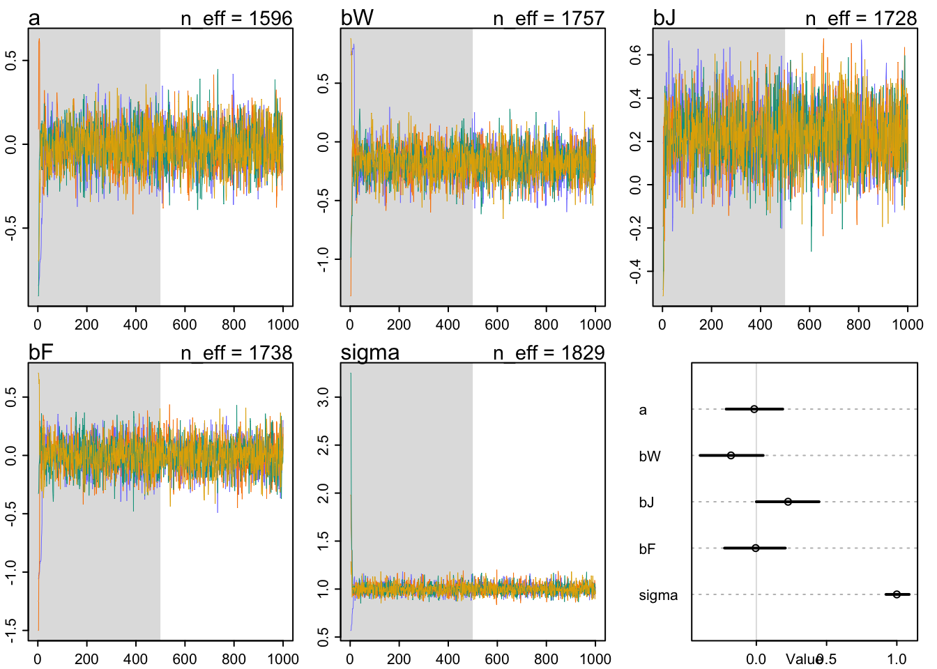
2.a INLA
d.i2a <- d %>%
  mutate(S = standardize(d$score),
    W = d$wine.amer,
    J = d$judge.amer,
    R= if_else(d$flight == "red", 1, 0))

m2a.i <- inla(S~W+J+R, data= d.i2a, control.fixed = list(
        mean= 0,
        prec= list(R=0.5, W=0.5, J= 0.5),
        mean.intercept= 0,
        prec.intercept= 0.2
),
control.compute = list(waic= TRUE))

summary(m2a.i)
##
## Call:
## c("inla(formula = S ~ W + J + R, data = d.i2a, control.compute =
## list(waic = TRUE), ", " control.fixed = list(mean = 0, prec = list(R =
## 0.5, W = 0.5, ", " J = 0.5), mean.intercept = 0, prec.intercept =
## 0.2))" )
## Time used:
## Pre = 1.29, Running = 0.205, Post = 0.193, Total = 1.69
## Fixed effects:
## mean sd 0.025quant 0.5quant 0.975quant mode kld
## (Intercept) -0.021 0.161 -0.336 -0.021 0.295 -0.021 0
## W -0.190 0.150 -0.486 -0.190 0.106 -0.190 0
## J 0.246 0.148 -0.045 0.246 0.538 0.246 0
## R -0.004 0.148 -0.294 -0.004 0.286 -0.004 0
##
## Model hyperparameters:
## mean sd 0.025quant 0.5quant
## Precision for the Gaussian observations 1.02 0.108 0.819 1.02
## 0.975quant mode
## Precision for the Gaussian observations 1.24 1.01
##
## Expected number of effective parameters(stdev): 3.96(0.004)
## Number of equivalent replicates : 45.42
##
## Watanabe-Akaike information criterion (WAIC) ...: 515.36
## Effective number of parameters .................: 4.79
##
## Marginal log-Likelihood: -274.11
## Posterior marginals for the linear predictor and
## the fitted values are computed## Pull out summaries from the model object
m1.i.sum <- summary(m1.i)
## Summarise results
m1.i.df <- data.frame(mean = m1.i.sum$fixed[,"mean"],
lower = m1.i.sum$fixed[,"0.025quant"],
upper = m1.i.sum$fixed[,"0.975quant"],
stringsAsFactors = FALSE)
mi.i.df <- bind_cols(as.factor(est), m1.i.df)## New names:
## * NA -> ...1m1.i.plot <- mi.i.df %>%
mutate(est= factor(est, levels= c("j.1", "j.2" , "j.3" , "j.4" , "j.5" ,"j.6" , "j.7" , "j.8" , "j.9" , "w.1" , "w.2" , "w.3" , "w.4" , "w.5" , "w.6" , "w.7" ,"w.8" , "w.9" ,"w.10" ,"w.11", "w.12" ,"w.13" ,"w.14", "w.15" ,"w.16", "w.17", "w.18", "w.19", "w.20"))) %>%
ggplot() +
geom_pointrange(aes(x = factor(est), y = mean, ymin = lower, ymax = upper), position = position_dodge(0.5)) +
xlab("coefficient") +
ylab("Estimate")+
coord_flip()+
theme_bw()
m1.i.plot 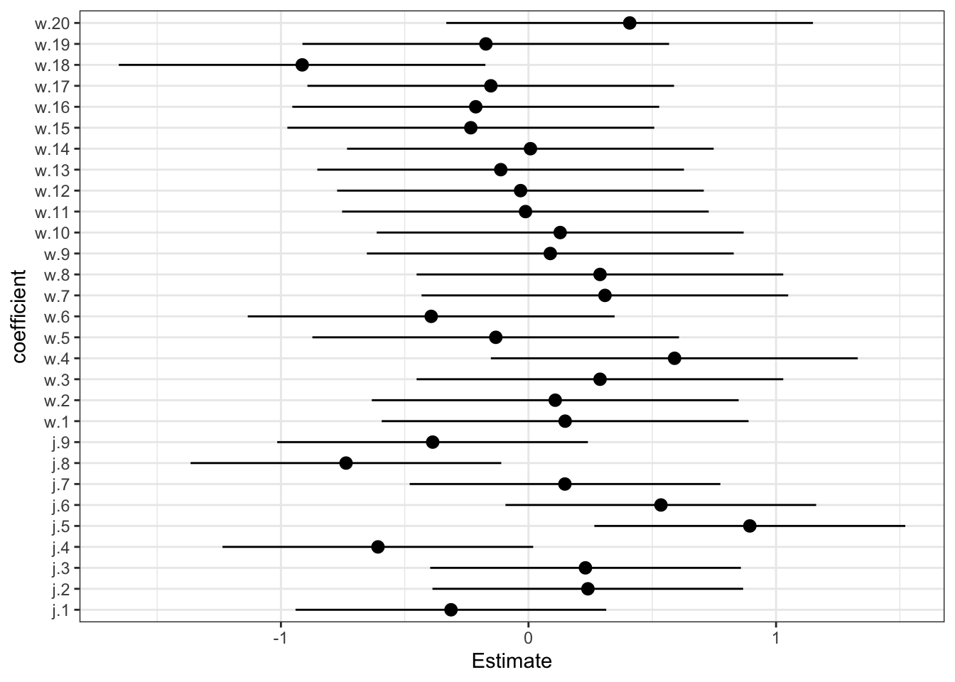 As expected, red and wines are on average the same—bR is right on top of zero. American judges seem to be more on average slightly more generous with ratings—bJ is slightly but reliably above zero. American wines have slightly lower average ratings than French wines—bW is mostly below zero, but not very large in absolute size.
2.b index variables
Okay, now for an index variable version. The thing about index variables is that you can easily end up with more parameters than in an equivalent indicator variable model. But it’s still the same posterior distribution. You can convert from one to the other (if the priors are also equivalent).
We’ll need three index variables: wid, jid, fid. Now wid is 1 for a French wine and 2 for a NJ wine,jid is 1 for a French judge and 2 for an American judge, and fid is 1 for red and 2 for white. Those 1L numbers are just the R way to type the number as an integer—“1L” is the integer 1, while “1” is the real number 1. We want integers for an index variable.
Now let’s think about priors for the parameters that correspond to each index value. Now the question isn’t how big the difference could be, but rather how far from the mean an indexed category could be. If we use Normal(0,0.5) priors, that would make a full standard deviation difference from the global mean rare. It will also match what we had above, in a crude sense. Again, I’d be tempted to something narrow, for the sake of regularization. But certainly something like Normal(0,10) is flat out silly, because it makes impossible values routine. Let’s see what we get:
2.b rethinking
dat_list2b <- list(
    S = standardize(d$score),
    wid = d$wine.amer + 1,
    jid = d$judge.amer + 1,
    fid= if_else(d$flight=="red",1L,2L)
    )

m2b <- ulam(
  alist(
    S ~ dnorm(mu, sigma),
    mu <- w[wid]+j[jid]+f[fid],
    w[wid]~ dnorm(0, 0.5),
    j[wid]~ dnorm(0, 0.5),
    f[wid]~ dnorm(0, 0.5),
  sigma ~ dexp(1)
    ), data=dat_list2b, chains=4 , cores=4
  )

precis(m2b, depth=2)
## mean sd 5.5% 94.5% n_eff Rhat4
## w[1] 0.0966267636 0.29498558 -0.3790303 0.5679111 952.8610 1.0027771
## w[2] -0.0858346645 0.29947353 -0.5696441 0.3905461 960.2548 1.0019704
## j[1] -0.1183499721 0.29633195 -0.6031432 0.3496110 1059.9772 1.0018204
## j[2] 0.1154412829 0.29126457 -0.3508953 0.5882257 1074.1928 1.0029881
## f[1] 0.0008060561 0.30871637 -0.4826726 0.5079951 784.3149 1.0026981
## f[2] 0.0043154703 0.30890116 -0.4659775 0.5120941 771.1461 1.0033839
## sigma 1.0016452222 0.05383488 0.9198169 1.0912787 1372.6385 0.9993503To see that this model is the same as the previous, let’s compute contrasts. The contrast between American and French wines is:
post <- extract.samples(m2b)
diff_w <- post$w[,2] - post$w[,1]
precis( diff_w )
## mean sd 5.5% 94.5% histogram
## diff_w -0.1824614 0.1421492 -0.416711 0.04384475 ▁▁▁▂▃▇▇▅▂▁▁That’s almost exactly the same mean and standard deviation as bW in the first model. The other contrasts match as well.
Something to notice about the two models is that the second one does sample less efficiently. The n_eff values are lower. This isn’t a problem, but it is a consequence of the higher correlations in the posterior, a result of the redundant parameterization. If you look at the pairs(m2b) plot, you’ll see tight correlations for each pair of index parameters of the same type. This is because really it is a difference that matters, and many combinations of two numbers can produce the same difference. But the priors keep this from ruining our inference. if you tried the same thing without priors, it would likely fall apart and return very large standard errors.
pairs(m2b)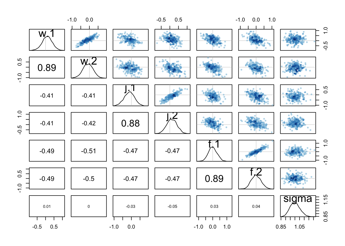
2.b INLA
Note that here we have used the selection argument to keep just the sampled values of the coefficients of wine.amer.no and wine.amer.yes. Note that the expression wine.amer.no = 1 means that we want to keep the first element in effect wine.amer.no. Note that in this case there is only a single value associated with wine.amer.no (i.e., the coefficient) but this can be extended to other latent random effects with possibly more values.
The object returned by inla.posterior.sample() is a list of length 100, where each element contains the samples of the different effects in the model in a name list.
Finally, function inla.posterior.sample.eval() is used to compute the product of the two coefficients. The output is a matrix with 1 row and 100 columns so that summary statistics can be computed from the posterior as usual:
d.i2b <- d %>%
  mutate(S = standardize(d$score),
   wine.amer.no= na_if(if_else(wine.amer==0, 1, 0), 0),
         wine.amer.yes= na_if(wine.amer, 0),
         judge.amer.no= na_if(if_else(judge.amer==0, 1, 0), 0),
         judge.amer.yes= na_if(judge.amer, 0),
         f.red= na_if(if_else(flight=="red", 1, 0), 0),
   f.white= na_if(if_else(flight=="white", 1, 0), 0)
         )


m2b.i<- inla(S~ -1 + wine.amer.no + wine.amer.yes + judge.amer.no+ judge.amer.yes + f.red + f.white, data= d.i2b,
                        control.fixed = list(
        mean= 0,
        prec= 0.5),
        control.compute = list(
          dic=TRUE, waic= TRUE, config=TRUE)
)

summary(m2b.i )
##
## Call:
## c("inla(formula = S ~ -1 + wine.amer.no + wine.amer.yes + judge.amer.no
## + ", " judge.amer.yes + f.red + f.white, data = d.i2b, control.compute
## = list(dic = TRUE, ", " waic = TRUE, config = TRUE), control.fixed =
## list(mean = 0, ", " prec = 0.5))")
## Time used:
## Pre = 1.39, Running = 0.244, Post = 0.245, Total = 1.87
## Fixed effects:
## mean sd 0.025quant 0.5quant 0.975quant mode kld
## wine.amer.no 0.097 0.821 -1.514 0.097 1.707 0.097 0
## wine.amer.yes -0.094 0.820 -1.703 -0.094 1.515 -0.094 0
## judge.amer.no -0.122 0.821 -1.733 -0.122 1.488 -0.122 0
## judge.amer.yes 0.126 0.820 -1.484 0.126 1.734 0.126 0
## f.red 0.000 0.820 -1.611 0.000 1.609 0.000 0
## f.white 0.004 0.820 -1.607 0.004 1.613 0.004 0
##
## Model hyperparameters:
## mean sd 0.025quant 0.5quant
## Precision for the Gaussian observations 1.02 0.108 0.819 1.02
## 0.975quant mode
## Precision for the Gaussian observations 1.24 1.01
##
## Expected number of effective parameters(stdev): 3.98(0.002)
## Number of equivalent replicates : 45.20
##
## Deviance Information Criterion (DIC) ...............: 515.53
## Deviance Information Criterion (DIC, saturated) ....: 188.15
## Effective number of parameters .....................: 5.07
##
## Watanabe-Akaike information criterion (WAIC) ...: 515.40
## Effective number of parameters .................: 4.81
##
## Marginal log-Likelihood: -274.88
## Posterior marginals for the linear predictor and
## the fitted values are computed## Pull out summaries from the model object
m2b.i.sum <- summary(m2b.i)
m2b.i.samp <- inla.posterior.sample(100, m2b.i , selection = list(wine.amer.no = 1, wine.amer.yes = 1))
m2b.i.contrast <- inla.posterior.sample.eval(function(...) {wine.amer.yes - wine.amer.no},
m2b.i.samp)## Warning in inla.posterior.sample.eval(function(...) {: Function
## 'inla.posterior.sample.eval()' is experimental.summary(as.vector(m2b.i.contrast))## Min. 1st Qu. Median Mean 3rd Qu. Max.
## -0.58772 -0.29199 -0.20004 -0.20118 -0.09873 0.140843. data(Wines2012) consider two-way interactions among the three features
Now consider two-way interactions among the three features.You should end up with three different interaction terms in your model. These will be easier to build, if you use indicator variables. Again use ulam, justify your priors, and be sure to check the chains. Explain what each interaction means. Be sure to interpret the model’s predictions on the outcome scale (mu, the expected score), not on the scale of individual parameters. You can use link to help with this, or just use your knowledge of the linear model instead. What do you conclude about the features and the scores? Can you relate the results of your model(s) to the individual judge and wine inferences from Problem 1?
Again I’ll show both the indicator approach and the index variable approach.
3.a indicator variables
3.a rethinking
For the indicator approach, we can use the same predictor variables as before, it’s the model that’s different. I used the same priors as before for the main effects. I used tighter priors for the interactions. Why? Because interactions represent sub-categories of data, and if we keep slicing up the sample, differences can’t keep getting bigger. Again, the most important thing is not to use flat priors like Normal(0,10) that produce impossible outcomes.
library(rethinking)
data(Wines2012)
d <- Wines2012

dat_list2 <- list(
    S = standardize(d$score),
    W = d$wine.amer,
    J = d$judge.amer,
    R= if_else(d$flight == "red", 1, 0))

m3a <- ulam(
  alist(
    S ~ dnorm(mu, sigma),
    mu <- a + bW*W + bJ*J + bR*R +
      bWJ*W*J + bWR*W*R + bJR*J*R,
    a ~ dnorm(0, 0.2),
   c(bW,bJ,bR) ~ dnorm(0,0.5),
    c(bWJ,bWR,bJR) ~ dnorm(0,0.25),
  sigma ~ dexp(1)
    ), data=dat_list2, chains=4 , cores=4)
## Error in open.connection(con, open = mode) :
## Timeout was reached: [github.com] Connection timed out after 10004 millisecondsprecis(m3a)## mean sd 5.5% 94.5% n_eff Rhat4
## a -0.05001514 0.13053594 -0.25735302 0.1583739 907.1065 0.9996431
## bR 0.08722749 0.18435834 -0.21952709 0.3821642 939.8246 0.9994441
## bJ 0.21311842 0.17777370 -0.06826854 0.5018780 1241.5379 1.0011227
## bW -0.07010677 0.17309924 -0.34546478 0.2055894 977.1175 1.0029427
## bJR 0.04492822 0.18317460 -0.24884781 0.3320738 1219.4018 1.0011258
## bWR -0.22580763 0.18009988 -0.50579686 0.0696629 1196.6973 1.0000129
## bWJ -0.03285475 0.17892221 -0.31443471 0.2560875 1280.9285 1.0025097
## sigma 0.99449691 0.05197665 0.91540590 1.0808165 1854.8918 1.0006698Reading the parameters this way is not easy. But right away you might notice that bW is now close to zero and overlaps it a lot on both sides. NJ wines are no longer on average worse. So the interactions did something. Glancing at the interaction parameters, you can see that only one of them has much mass away from zero, bWR, the interaction between NJ wines and red flight, so red NJ wines. To get the predicted scores for red and white wines from both NJ and France, for both types of judges, we can use link:
pred_dat <- data.frame(
    W = rep( 0:1 , times=4 ),
    J = rep( 0:1 , each=4 ),
    R = rep( c(0,0,1,1) , times=2 )
)
mu <- link( m3a )

row_labels <- paste( ifelse(pred_dat$W==1,"A","F") ,
                 ifelse(pred_dat$J==1,"A","F") ,
                 ifelse(pred_dat$R==1,"R","W") , sep="" )

plot( precis( list(mu=mu) , 2 ) , labels=row_labels )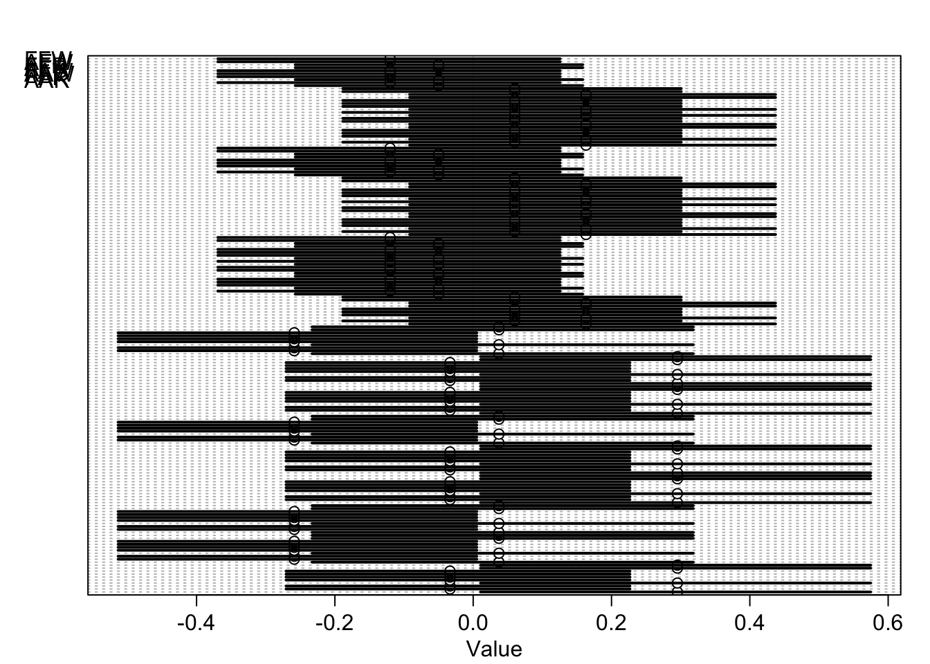
3.a INLA
library(INLA)
library(rethinking)
library(tidyverse)
data(Wines2012)
d <- Wines2012

#we want to predict the score for each combination of factors.
pred_dat <- data.frame(S= NA,
    W = rep( 0:1 , times=4 ),
    J = rep( 0:1 , each=4 ),
    R = rep( c(0,0,1,1) , times=2 )
    )

d.i3a <- d %>%
  mutate(S = standardize(d$score),
    W = d$wine.amer,
    J = d$judge.amer,
    R= if_else(d$flight == "red", 1, 0)) %>%
  select(c("S", "W", "J", "R")) %>%
  rbind(pred_dat)


#indices of the scores with missing values
d.i.3na <- which(is.na(d.i3a$S))

m3a.i <- inla(S~W+J+R+ W*J + W*R + J*R, data= d.i3a,

              control.fixed = list(
        mean= 0,
        prec= list(R=1/(0.5^2), W=1/(0.5^2), J= 1/(0.5^2), WJ = 1/(0.25^2), WR=1/(0.25^2), JR= 1/(0.25^2)),
        mean.intercept= 0,
        prec.intercept= 1/(0.2^2)
),
control.compute = list(config= TRUE, waic= TRUE),
control.predictor=list(compute=TRUE),
)

summary(m3a.i)
##
## Call:
## c("inla(formula = S ~ W + J + R + W * J + W * R + J * R, data = d.i3a,
## ", " control.compute = list(config = TRUE, waic = TRUE),
## control.predictor = list(compute = TRUE), ", " control.fixed =
## list(mean = 0, prec = list(R = 1/(0.5^2), ", " W = 1/(0.5^2), J =
## 1/(0.5^2), WJ = 1/(0.25^2), WR = 1/(0.25^2), ", " JR = 1/(0.25^2)),
## mean.intercept = 0, prec.intercept = 1/(0.2^2)))" )
## Time used:
## Pre = 1.51, Running = 0.23, Post = 0.265, Total = 2
## Fixed effects:
## mean sd 0.025quant 0.5quant 0.975quant mode kld
## (Intercept) -0.073 0.138 -0.344 -0.073 0.199 -0.073 0
## W 0.039 0.207 -0.368 0.039 0.445 0.040 0
## J 0.156 0.215 -0.267 0.156 0.577 0.157 0
## R 0.178 0.225 -0.264 0.178 0.618 0.179 0
## W:J -0.023 0.267 -0.548 -0.023 0.503 -0.023 0
## W:R -0.494 0.270 -1.025 -0.494 0.038 -0.494 0
## J:R 0.142 0.271 -0.389 0.141 0.673 0.141 0
##
## Model hyperparameters:
## mean sd 0.025quant 0.5quant
## Precision for the Gaussian observations 1.03 0.109 0.825 1.02
## 0.975quant mode
## Precision for the Gaussian observations 1.25 1.02
##
## Expected number of effective parameters(stdev): 5.96(0.064)
## Number of equivalent replicates : 30.18
##
## Watanabe-Akaike information criterion (WAIC) ...: 516.02
## Effective number of parameters .................: 6.84
##
## Marginal log-Likelihood: -281.65
## Posterior marginals for the linear predictor and
## the fitted values are computed#names of predicted scores
row_labels <- paste( ifelse(pred_dat$W==1,"Aw","Fw") ,
ifelse(pred_dat$J==1,"Aj","Fj") ,
ifelse(pred_dat$R==1,"Red","Wh") , sep="" )
m3a.i.postmean <- bind_cols(label= row_labels, m3a.i$summary.linear.predictor[d.i.3na, ]) %>%
select(c("label", "mean", "sd", "0.025quant", "0.975quant"))
names(m3a.i.postmean) <- c("label", "mean", "sd", "LCI", "UCI")
m3a.i.postmean.plot <- ggplot(data= m3a.i.postmean, aes(y=label, x=mean, label=label)) +
geom_point(size=4, shape=19) +
geom_errorbarh(aes(xmin=LCI, xmax=UCI), height=.3) +
coord_fixed(ratio=.3) +
geom_vline(xintercept=0, linetype='longdash') +
theme_bw()
m3a.i.postmean.plot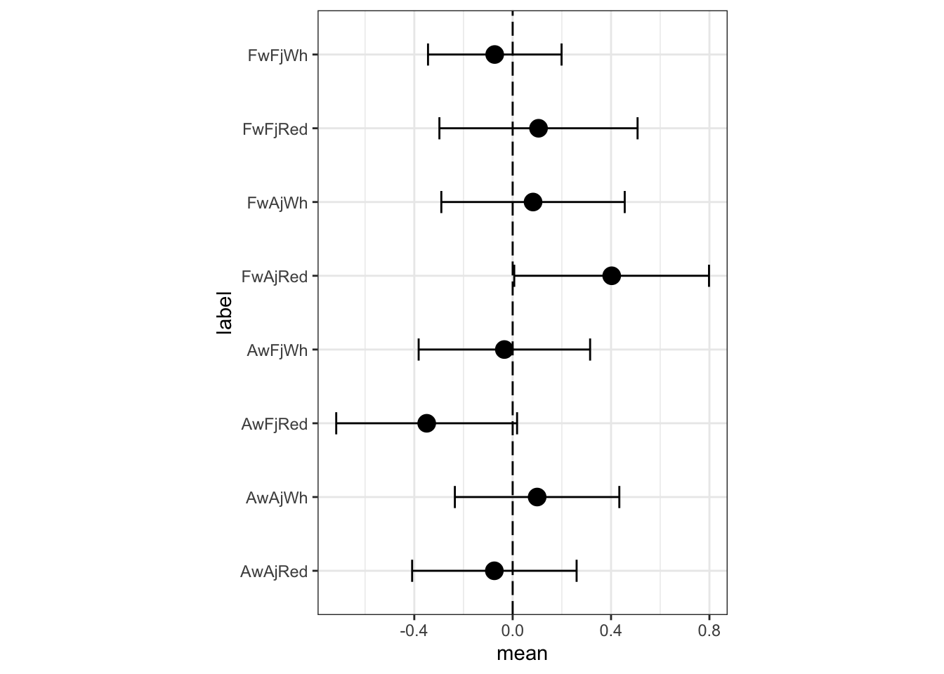
3.b index variables
Now let’s do an index version. The way to think of this is to make unique parameters for each combination. If we consider all the interactions—including a three-way interaction between nation, judge and flight—there would be 8 combinations and so 8 parameters to estimate. Let’s go ahead and do that, so we can simultaneously consider the 3-way interaction.
3.b rethinking
There are several ways to go about coding this. I’m going to use a trick and make an array of parameters. An array is like a matrix, but can have more than 2 dimensions. If we make a 2-by-2-by-2 array of parameters, then there will be 8 parameters total and we can access each by just using these index variables.
dat_list2b <- list(
    S = standardize(d$score),
    wid = d$wine.amer + 1,
    jid = d$judge.amer + 1,
    fid= if_else(d$flight=="red",1L,2L)
    )

d3 <- data.frame(dat_list2b)
** in rethinking::ulam** The ‘2,2,2’ literal is not very elegant, so I’m likely to improve this is a later version. Either way, the result is displayed on the next page (for sake of line breaks).
#in ulam

m3b <- ulam(
    alist(
        S ~ dnorm( mu , sigma ),
        mu <- w[wid,jid,fid],
        real['2,2,2']:w ~ normal(0,0.5),
        sigma ~ dexp(1)
    ), data=dat_list2b , chains=4 , cores=4 )

precis(m3b, depth=3)
## mean sd 5.5% 94.5% n_eff Rhat4
## w[1,1,1] 0.21103673 0.22267977 -0.13953197 0.56826400 2676.031 1.0009000
## w[1,1,2] -0.30250094 0.21912327 -0.66287409 0.03867354 2167.897 1.0017658
## w[1,2,1] 0.26832815 0.20625809 -0.06452683 0.59679971 2999.359 0.9991988
## w[1,2,2] 0.16456930 0.21086740 -0.17184942 0.49783080 2703.213 1.0009935
## w[2,1,1] -0.36746897 0.18678822 -0.65644415 -0.05561319 2110.281 1.0013134
## w[2,1,2] 0.03746607 0.18865657 -0.26167238 0.33322569 2309.842 0.9986979
## w[2,2,1] -0.01969343 0.16719165 -0.29333425 0.25140293 2546.988 0.9992449
## w[2,2,2] 0.04023122 0.16954093 -0.22832951 0.31352833 2881.246 0.9997324
## sigma 0.99060862 0.05245158 0.91038839 1.08003757 2263.957 0.9997073row_labels = c("FFR","FFW","FAR","FAW","AFR","AFW","AAR","AAW" )
plot( precis( m3b , 3 , pars="w" ) , labels=row_labels )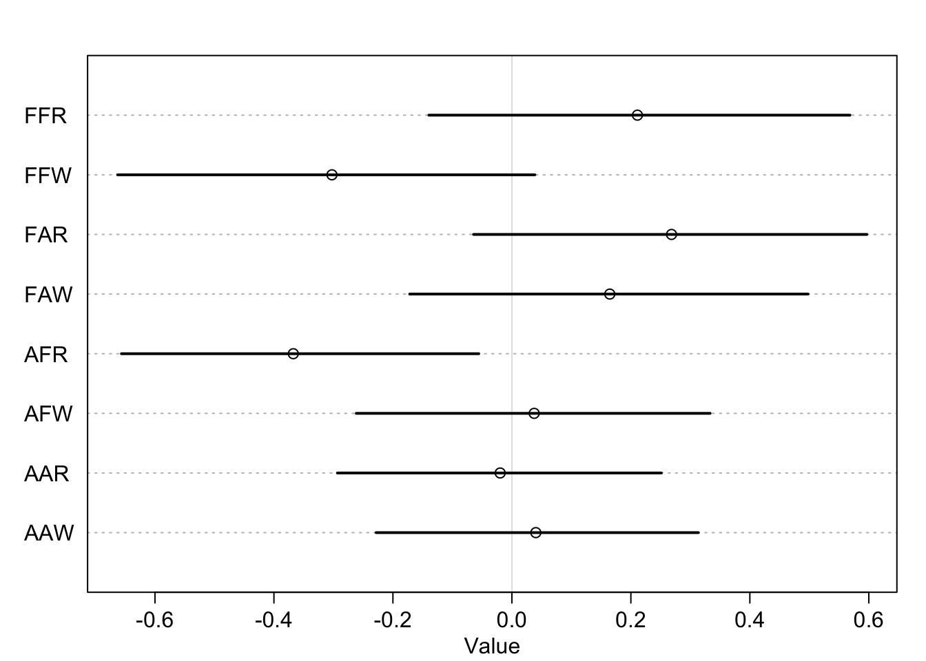
3.b INLA
Note that here we have used the selection argument to keep just the sampled values of the coefficients of wine.amer.no and wine.amer.yes. Note that the expression wine.amer.no = 1 means that we want to keep the first element in effect wine.amer.no. Note that in this case there is only a single value associated with wine.amer.no (i.e., the coefficient) but this can be extended to other latent random effects with possibly more values.
The object returned by inla.posterior.sample() is a list of length 100, where each element contains the samples of the different effects in the model in a name list.
Finally, function inla.posterior.sample.eval() is used to compute the product of the two coefficients. The output is a matrix with 1 row and 100 columns so that summary statistics can be computed from the posterior as usual:
library(INLA)
library(rethinking)
library(tidyverse)
data(Wines2012)
d <- Wines2012

#names of predicted scores
row_labels <- paste( ifelse(pred_dat$W==1,"Aw","Fw") ,
ifelse(pred_dat$J==1,"Aj","Fj") ,
ifelse(pred_dat$R==1,"Red","Wh") , sep="" )

d3b.i <- d %>%
  mutate(S = standardize(d$score),
    W = d$wine.amer,
    J = d$judge.amer,
    R= if_else(d$flight == "red", 1, 0)) %>%
  mutate(index= paste(ifelse(W==1,"Aw","Fw") ,
ifelse(J==1,"Aj","Fj") ,
ifelse(R==1,"Red","Wh"), sep="" ),
value= 1) %>%
  spread(index, value)


labels <- paste( ifelse(d3b.i$W==1,"Aw","Fw"),
ifelse(d3b.i$J==1,"Aj","Fj") ,
ifelse(d3b.i$R==1,"Red","Wh") , sep="" )


m3b.i<- inla(S~ -1 + FwFjRed +FwFjWh+ FwAjRed+ FwAjWh + AwFjRed + AwFjWh +AwAjRed + AwAjWh, data= d3b.i,
                        control.fixed = list(
        mean= 0,
        prec= 1/(0.5^2)),
        control.compute = list(
          dic=TRUE, waic= TRUE, config=TRUE)
)

summary(m3b.i)
##
## Call:
## c("inla(formula = S ~ -1 + FwFjRed + FwFjWh + FwAjRed + FwAjWh + ", "
## AwFjRed + AwFjWh + AwAjRed + AwAjWh, data = d3b.i, control.compute =
## list(dic = TRUE, ", " waic = TRUE, config = TRUE), control.fixed =
## list(mean = 0, ", " prec = 1/(0.5^2)))")
## Time used:
## Pre = 1.5, Running = 0.212, Post = 0.265, Total = 1.98
## Fixed effects:
## mean sd 0.025quant 0.5quant 0.975quant mode kld
## FwFjRed 0.204 0.221 -0.231 0.204 0.637 0.204 0
## FwFjWh -0.306 0.221 -0.739 -0.306 0.129 -0.307 0
## FwAjRed 0.267 0.202 -0.130 0.267 0.663 0.268 0
## FwAjWh 0.165 0.202 -0.232 0.165 0.561 0.165 0
## AwFjRed -0.361 0.187 -0.727 -0.361 0.007 -0.361 0
## AwFjWh 0.036 0.187 -0.331 0.036 0.403 0.036 0
## AwAjRed -0.017 0.169 -0.349 -0.017 0.316 -0.017 0
## AwAjWh 0.039 0.169 -0.294 0.039 0.371 0.039 0
##
## Model hyperparameters:
## mean sd 0.025quant 0.5quant
## Precision for the Gaussian observations 1.04 0.111 0.833 1.03
## 0.975quant mode
## Precision for the Gaussian observations 1.27 1.03
##
## Expected number of effective parameters(stdev): 6.78(0.115)
## Number of equivalent replicates : 26.57
##
## Deviance Information Criterion (DIC) ...............: 515.07
## Deviance Information Criterion (DIC, saturated) ....: 190.96
## Effective number of parameters .....................: 7.87
##
## Watanabe-Akaike information criterion (WAIC) ...: 515.00
## Effective number of parameters .................: 7.49
##
## Marginal log-Likelihood: -269.20
## Posterior marginals for the linear predictor and
## the fitted values are computedm3b.i.postmean <- m3b.i$summary.fixed %>%
rownames_to_column( "label") %>%
select(c("label", "mean", "sd", "0.025quant", "0.975quant"))
names(m3b.i.postmean) <- c("label", "mean", "sd", "LCI", "UCI")
m3b.i.postmean.plot <- ggplot(data= m3b.i.postmean, aes(y=label, x=mean, label=label)) +
geom_point(size=4, shape=19) +
geom_errorbarh(aes(xmin=LCI, xmax=UCI), height=.3) +
coord_fixed(ratio=.3) +
geom_vline(xintercept=0, linetype='longdash') +
theme_bw()
m3b.i.postmean.plot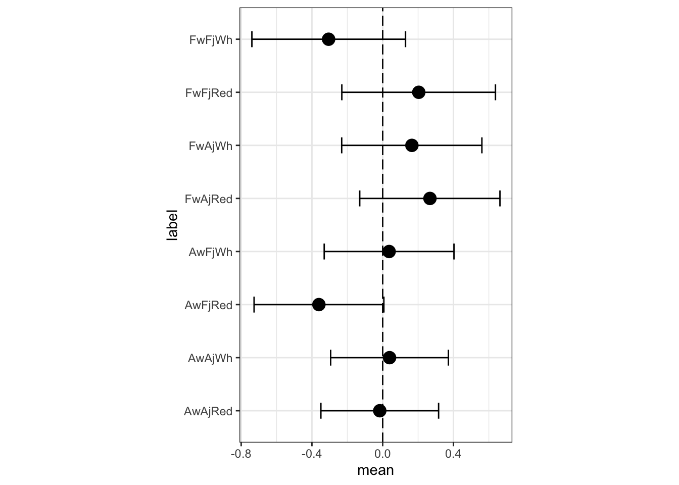
The previous predictions, for comparison:
m3a.i.postmean.plot
The most noticeable change is that FFW (French wines, French judges, white) have a lower expected rating in the full interaction model. There are some other minor differences as well. What has happened? The three way interaction would be, in the first model’s indicator terms, when a wine is American, the judge is American, and the flight is red. In the first model, a prediction for such a wine is just a sum of parameters:
μi =α+βW +βJ +βR +βWJ +βWR +βJR
This of course limits means that these parameters have to account for the AAR wine. In the full interaction mode, an AAR wine gets its own parameter, as does every other combination. None of the parameters get polluted by averaging over different combinations. Of course, there isn’t a lot of evidence that prediction is improved much by allowing this extra parameter. The differences are small, overall. These wines are all quite good. But it is worth understand how the full interaction model gains additional flexibility. This additional flexibility typically requires some addition regularization. When we arrive at multilevel models later, you’ll see how we can handle regularization more naturally inside of a model.